Basic elements of an IMAGINE pipeline
In this tutorial, we focus on introducing the basic building blocks of the IMAGINE package and how to use them for assembling a Bayesian analysis pipeline.
We will use mock data with only two independent free parameters. First, we will generate the mock data. Then we will assemble all elements needed for the IMAGINE pipeline, execute the pipeline and investigate its results.
The mock data are designed to “naively” mimic Faraday depth, which is affected linearly by the (Galactic) magnetic field and thermal electron density. As a function of position \(x\), we define a constant coherent magnetic field component \(a_0\) and a random magnetic field component which is drawn from a Gaussian distribution with standard deviation \(b_0\). The electron density is assumed to be independently known and given by a \(\cos(x)\) with arbitrary scaling. The mock data values we get are related to the Faraday depth of a background source at some arbitrary distance:
where \(\{a_0,b_0\}\) is the ‘physical’ parameter set, and \(s\) represents the seed for random variable generation.
The purpose is not to fit the exact signal, since it includes a stochastic component, but to fit the amplitude of the signal and of the variations around it. So this is fitting the strength of the coherent field \(a_0\) and the amplitude of the random field \(b_0\). With these mock data and its (co)variance matrix, we shall assemble the IMAGINE pipeline, execute it and examine its results.
First, import the necessary packages.
[1]:
import numpy as np
import astropy.units as u
import astropy as apy
import matplotlib.pyplot as plt

import imagine as img

%matplotlib inline
1) Preparing the mock data
In calculating the mock data values, we introduce noise as:
For simplicity, we propose a simple gaussian noise with mean zero and a standard deviation \(e\):
.
We will assume that we have 10 points in the x-direction, in the range \([0, 2\pi]\,\rm kpc\).
[2]:
a0 = 3. # true value of a in microgauss
b0 = 6. # true value of b in microgauss
e = 0.1 # std of gaussian measurement error
s = 233 # seed fixed for signal field

size = 10 # data size in measurements
x = np.linspace(0.01,2.*np.pi-0.01,size) # where the observer is looking at

np.random.seed(s) # set seed for signal field

signal = (1+np.cos(x)) * np.random.normal(loc=a0,scale=b0,size=size)

fd = signal + np.random.normal(loc=0.,scale=e,size=size)

# We load these to an astropy table for illustration/visualisation
data = apy.table.Table({'meas' : u.Quantity(fd, u.microgauss*u.cm**-3),
                  'err': np.ones_like(fd)*e,
                  'x': x,
                  'y': np.zeros_like(fd),
                  'z': np.zeros_like(fd),
                  'other': np.ones_like(fd)*42})
data[:4] # Shows the first 4 points in tabular form
[2]:
| meas | err | x | y | z | other |
|---|---|---|---|---|---|
| uG / cm3 | |||||
| float64 | float64 | float64 | float64 | float64 | float64 |
| 16.4217790817552 | 0.1 | 0.01 | 0.0 | 0.0 | 42.0 |
| 7.172468731201507 | 0.1 | 0.7059094785755097 | 0.0 | 0.0 | 42.0 |
| -3.2254947821460433 | 0.1 | 1.4018189571510193 | 0.0 | 0.0 | 42.0 |
| 0.27949334758966465 | 0.1 | 2.0977284357265287 | 0.0 | 0.0 | 42.0 |
These data need to be converted to an IMAGINE compatible format. To do this, we first create TabularDataset object, which helps importing dictionary-like dataset onto IMAGINE.
[3]:
mockDataset = img.observables.TabularDataset(data, name='test',
                                             data_col='meas',
                                             err_col='err')
These lines simply explain how to read the tabular dataset (note that the ‘other’ column is ignored): name contains the type of observable we are using (here, we use ‘test’, it could also be ‘sync’ for synchrotron observables (e.g, Stokes parameters), ‘fd’ for Faraday Depth, etc. The data_col argument specifies the key or name of the column containing the relevant measurement. Coordinates (coords_type) can be given in either 'cartesian' or 'galactic'. If not provided, the
coordinates type is derived from the provided data. In this example, we provided \(x\), \(y\) and \(z\) in \(\rm kpc\) and therefore the coordinates type is assumed to be ‘cartesian’. The units of the dataset are represented using astropy.units objects and can be supplied (if they are, the Simulator will later check whether these are adequate and automatically convert the data to other units if needed).
The dataset can be loaded onto a Measurements object, which is subclass of ObservableDict. This object allows one to supply multiple datasets to the pipeline.
[4]:
# Create Measurements object using mockDataset
mock_data = img.observables.Measurements(mockDataset)
The dataset object creates a standard key for each appended dataset. In our case, there is only one key.
[5]:
keys = list(mock_data.keys())
keys
[5]:
[('test', None, 'tab', None)]
Let us plot the mock data as well as the \(1+\cos(x)\) function that is the underlying variation.
The property Measurements.global_data extracts arrays from the Observable object which is hosted inside the ObservableDict class.
[6]:
plt.scatter(x, mock_data[keys[0]].global_data[0], marker='.', label='signal')
plt.plot(x,(1+np.cos(x))*a0,'r--',label='$1+\cos(x)$')
plt.xlabel('x'); plt.legend();
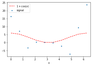
Note that the variance in the signal is highest where the \(\cos(x)\) is also strongest. This is the way we expect the Faraday depth to work, since a fluctuation in the strength of \(\mathbf B\) has a larger effect on the RM when \(n_e\) also happens to be higher.
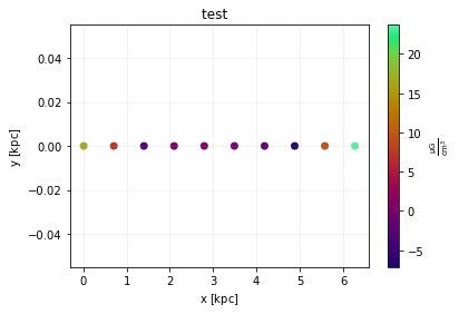
IMAGINE also comes with a built-in method for showing the contents of a Measurements objects on a skymap. In the next cell this is exemplified, though not very useful for this specific example.
[7]:
mock_data.show(cartesian_axes='xy')
2) Pipeline assembly
Now that we have generated mock data, there are a few steps to set up the pipeline to estimate the input parameters. We need to specify: a grid, Field Factories, Simulators, and Likelihoods.
Setting the coordinate grid
Fields in IMAGINE represent models of any kind of physical field – in this particular tutorial, we will need a magnetic field and thermal electron density.
The Fields are evaluated on a grid of coordinates, represented by a img.Grid object. Here we exemplify how to produce a regular cartesian grid. To do so, we need to specify the values of the coordinates on the 6 extremities of the box (i.e. the minimum and maximum value for each coordinate), and the resolution over each dimension.
For this particular artificial example, we actually only need one dimension, so we set the resolution to 1 for \(y\) and \(z\).
[8]:
one_d_grid = img.fields.UniformGrid(box=[[0,2*np.pi]*u.kpc,
                                         [0,0]*u.kpc,
                                         [0,0]*u.kpc],
                                    resolution=[30,1,1])
Preparing the Field Factory list
A particular realisation of a model for a physical field is represented within IMAGINE by a Field object, which, given set of parameters, evaluates the field for over the grid.
A Field Factory is an associated piece of infrastructure used by the Pipeline to produce new Fields. It is a Factory object that needs to be initialized and supplied to the Pipeline. This is what we will illustrate here.
[9]:
from imagine import fields
ne_factory = fields.CosThermalElectronDensityFactory(grid=one_d_grid)
The previous line instantiates CosThermalElectronDensityFactory with the previously defined Grid object. This Factory allows the Pipeline to produce CosThermalElectronDensity objects. These correspond to a toy model for electron density with the form:
We can set and check the default parameter values in the following way:
[10]:
ne_factory.default_parameters= {'a': 1*u.rad/u.kpc,
                                'beta':  np.pi/2*u.rad,
                                'gamma': np.pi/2*u.rad}
ne_factory.default_parameters
[10]:
{'n0': <Quantity 1. 1 / cm3>,
 'a': <Quantity 1. rad / kpc>,
 'b': <Quantity 0. rad / kpc>,
 'c': <Quantity 0. rad / kpc>,
 'alpha': <Quantity 0. rad>,
 'beta': <Quantity 1.57079633 rad>,
 'gamma': <Quantity 1.57079633 rad>}
[11]:
ne_factory.active_parameters
[11]:
()
For ne_factory, no active parameters were set. This means that the Field will be always evaluated using the specified default parameter values.
We will now similarly define the magnetic field, using the NaiveGaussianMagneticField which constructs a “naive” random field (i.e. the magnitude of \(x\), \(y\) and \(z\) components of the field are drawn from a Gaussian distribution without imposing zero divergence, thus do not use this for serious applications).
[12]:
B_factory = fields.NaiveGaussianMagneticFieldFactory(grid=one_d_grid)
Differently from the case of ne_factory, in this case we would like to make the parameters active. All individual components of the field are drawn from a Gaussian distribution with mean \(a_0\) and standard deviation \(b_0\). To set these parameters as active we do:
[13]:
B_factory.active_parameters = ('a0','b0')
B_factory.priors ={'a0': img.priors.FlatPrior(xmin=-4*u.microgauss,
                                              xmax=5*u.microgauss),
                   'b0': img.priors.FlatPrior(xmin=2*u.microgauss,
                                              xmax=10*u.microgauss)}
In the lines above we chose uniform (flat) priors for both parameters within the above specified ranges. Any active parameter must have a Prior distribution specified.
Once the two FieldFactory objects are prepared, they put together in a list which is later supplied to the Pipeline.
[14]:
factory_list = [ne_factory, B_factory]
Initializing the Simulator
For this tutorial, we use a customized TestSimulator which simply computes the quantity: \(t(x,y,z) = B_y\,n_e\,\),i.e. the contribution at one specific point to the Faraday depth.
The simulator is initialized with the mock Measurements defined before, which allows it to know what is the correct format for output.
[15]:
from imagine.simulators import TestSimulator
simer = TestSimulator(mock_data)
Initializing the Likelihood
IMAGINE provides the Likelihood class with EnsembleLikelihood and SimpleLikelihood as two options. The SimpleLikelihood is what you expect, computing a single \(\chi^2\) from the difference of the simulated and the measured datasets. The EnsembleLikelihood is how IMAGINE handles a signal which itself includes a stochastic component, e.g., what we call the Galactic variance. This likelihood module makes use of a finite ensemble of simulated realizations and uses their mean
and covariance to compare them to the measured dataset.
[16]:
likelihood = img.likelihoods.EnsembleLikelihood(mock_data)
3) Running the pipeline
Now we have all the necessary components available to run our pipeline. This can be done through a Pipeline object, which interfaces with some algorithm to sample the likelihood space accounting for the prescribed prior distributions for the parameters.
IMAGINE comes with a range of samplers coded as different Pipeline classes, most of which are based on the nested sampling approach. In what follows we will use the MultiNest sampler as an example.
IMAGINE takes care of stochastic fields by evaluating an ensemble of random realisations for each selected point in the parameter space, and computing the associated covariance (i.e. estimating the Galactic variance). We can set this up through the ensemble_size argument.
Now we are ready to initialize our final pipeline.
[17]:
pipeline = img.pipelines.MultinestPipeline(simulator=simer,
                                           run_directory='../runs/tutorial_one',
                                           factory_list=factory_list,
                                           likelihood=likelihood,
                                           ensemble_size=27)
The run_directory keyword is used to setup where the state of the pipeline is saved (allowing loading the pipeline in the future). It is also where the chains generated by the sampler are saved in the sampler’s native format (if the sampler supports this).
The property sampling_controllers allows one to send sampler-specific parameters to the chosen Pipeline. Each IMAGINE Pipeline object will have slightly different sampling controllers, which can be found in the specific Pipeline’s docstring.
[18]:
pipeline.sampling_controllers = {'evidence_tolerance': 0.5, 'n_live_points': 200}
In a standard nested sampling approach, a set of “live points” is initially sampled from the prior distribution. After each iteration the point with the smallest likelihood is removed (it becomes a dead point, and its likelihood value is stored) and a new point is sampled from the prior. As each dead point is associated to some prior volume, they can be used to estimate the evidence (see, e.g. here for details). In
the MultinestPipeline, the number of live points is set using the 'n_live_points' sampling controller.
The sampling parameter 'evidence_tolerance' allows one to control the target error in the estimated evidence.
Now, we finally can run the pipeline!
[19]:
results = pipeline()
analysing data from ../runs/tutorial_one/chains/multinest_.txt
Thus, one can see that after the pipeline finishes running, a brief summary report is written to screen.
When one runs the pipeline it returns a results dictionary object in the native format of the chosen sampler. Alternatively, after running the pipeline object, the results can also be accessed through its attributes, which are standard interfaces (i.e. all pipelines should work in the same way).
For comparing different models, the quantity of interest is the model evidence (or marginal likelihood) \(\mathcal Z\). After a run, this can be easily accessed as follows.
[20]:
print('log evidence: {0:.2f} ± {1:.2f}'.format(pipeline.log_evidence,
                                               pipeline.log_evidence_err))
log evidence: -33.74 ± 0.07
A dictionary containing a summary of the constraints to the parameters can be accessed through the property posterior_summary:
[21]:
pipeline.posterior_summary
[21]:
{'naive_gaussian_magnetic_field_a0': {'median': <Quantity 3.04653036 uG>,
  'errlo': <Quantity 2.09241063 uG>,
  'errup': <Quantity 1.26013795 uG>,
  'mean': <Quantity 2.62797986 uG>,
  'stdev': <Quantity 1.73790351 uG>},
 'naive_gaussian_magnetic_field_b0': {'median': <Quantity 6.09011278 uG>,
  'errlo': <Quantity 1.15964546 uG>,
  'errup': <Quantity 1.61955049 uG>,
  'mean': <Quantity 6.2845587 uG>,
  'stdev': <Quantity 1.37869584 uG>}}
In most cases, however, one would (should) prefer to work directly on the samples produced by the sampler. A table containing the parameter values of the samples generated can be accessed through:
[22]:
samples = pipeline.samples
samples[:3] # Displays only first 3 rows
[22]:
| naive_gaussian_magnetic_field_a0 | naive_gaussian_magnetic_field_b0 |
|---|---|
| uG | uG |
| float64 | float64 |
| -3.3186057209968567 | 5.630247116088867 |
| -3.163660407066345 | 6.178023815155029 |
| 4.913007915019989 | 3.289425849914551 |
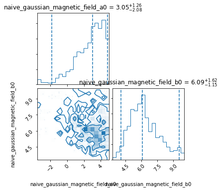
For convenience, the corner plot showing the posterior distribution obtained from the samples can be generated using the corner_plot method of the Pipeline object (which uses the corner library). This can show “truth” values of the parameters (in case someone is doing a test like this one).
[23]:
pipeline.corner_plot(truths_dict={'naive_gaussian_magnetic_field_a0': 3,
                                  'naive_gaussian_magnetic_field_b0': 6});

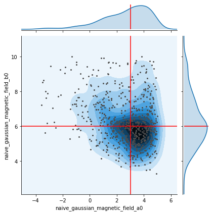
One can, of course, choose other plotting/analysis routines. Below, the use of seaborn is exemplified.
[24]:
import seaborn as sns
def plot_samples_seaborn(samp):

    def show_truth_in_jointplot(jointplot, true_x, true_y, color='r'):
        for ax in (jointplot.ax_joint, jointplot.ax_marg_x):
            ax.vlines([true_x], *ax.get_ylim(), colors=color)
        for ax in (jointplot.ax_joint, jointplot.ax_marg_y):
            ax.hlines([true_y], *ax.get_xlim(), colors=color)

    snsfig = sns.jointplot(*samp.colnames, data=samp.to_pandas(), kind='kde')
    snsfig.plot_joint(sns.scatterplot, linewidth=0, marker='.', color='0.3')
    show_truth_in_jointplot(snsfig, a0, b0)
[25]:
plot_samples_seaborn(samples)
Random seeds and convergence checks
The pipeline relies on random numbers in multiple ways. The Monte Carlo sampler will draw randomly chosen points in the parameter space duing its exploration (in the specific case of nested sampling pipelines, these are drawn from the prior distributions). Also, while evaluating the fields at each point, random realisations of the stochastic fields are generated.
It is possible to control the behaviour of the random seeding of an IMAGINE pipeline through the attribute master_seed. This attribute has two uses: it is passed to the sampler, ensuring that its behaviour is reproducible; and it is also used to generate a fresh list of new random seeds to each stochastic field that is evaluated.
[26]:
pipeline.master_seed
[26]:
1
By default, the master seed is fixed and set to 1, but you can alter its value before running the pipeline.
One can also change the seeding behaviour through the random_type attribute. There are three allowed options for this:
- ‘controllable’ - the
master_seedis constant and a re-running the pipeline should lead to the exact same results (default), and the random seeds which are used for generating the ensembles of stochastic fields are drawn in the beginning of the pipeline run; - ‘free’ - on each execution, a new
master_seedis drawn (using numpy.randint), moreover: at each evaluation of the likelihood the stochastic fields receive a new set of ensemble seeds; - ‘fixed’ - this mode is for debugging purposes. The
master_seedis fixed, as in the ‘controllable’ case, however each individual stochastic field receives the exact same list of ensemble seeds every time (while in thecontrollablethese are chosen “randomly” at run-time). Such choice can be inspected usingpipeline.ensemble_seeds.
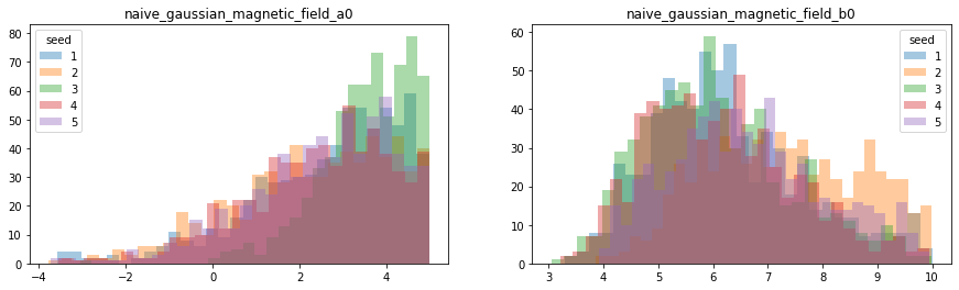
Let us now check whether different executions of the pipeline are generating consistent results. To do so, we run it five times and just overplot histograms of the outputs to see if they all look the same. The following can be done in a few minutes.
[27]:
fig, axs = plt.subplots(1, 2, figsize=(15, 4))
repeat = 5
pipeline.show_summary_reports = False  # Avoid summary reports
pipeline.sampling_controllers['resume'] = False # Pipeline will re-run
samples_list = []
for i in range(1,repeat+1):
    print('-'*60+'\nRun {}/{}'.format(i,repeat))
    if i>1:
        # Re-runs the pipeline with a different seed
        pipeline.master_seed = i
        _ = pipeline()
    print('log Z = ', round(pipeline.log_evidence,4),
          '±', round(pipeline.log_evidence_err,4))

    samples = pipeline.samples

    for j, param in enumerate(pipeline.samples.columns):
        samp = samples[param]
        axs[j].hist(samp.value, alpha=0.4, bins=30, label=pipeline.master_seed)
        axs[j].set_title(param)
    # Stores the samples for later use
    samples_list.append(samples)

for i in range(2):
    axs[i].legend(title='seed')
------------------------------------------------------------
Run 1/5
log Z =  -33.7403 ± 0.0686
------------------------------------------------------------
Run 2/5
  analysing data from ../runs/tutorial_one/chains/multinest_.txt
log Z =  -36.422 ± 0.0599
------------------------------------------------------------
Run 3/5
  analysing data from ../runs/tutorial_one/chains/multinest_.txt
log Z =  -33.593 ± 0.0788
------------------------------------------------------------
Run 4/5
  analysing data from ../runs/tutorial_one/chains/multinest_.txt
log Z =  -33.329 ± 0.0636
------------------------------------------------------------
Run 5/5
  analysing data from ../runs/tutorial_one/chains/multinest_.txt
log Z =  -34.6659 ± 0.0663
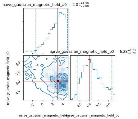
After being satisfied, one may want to put together all the samples. A set of rigorous tools for combining multiple pipelines/runs is currently under development, but a first order approximation to this can be seen below:
[28]:
all_samples = apy.table.vstack(samples_list)
img.tools.corner_plot(table=all_samples,
                      truths_dict={'naive_gaussian_magnetic_field_a0': 3,
                                   'naive_gaussian_magnetic_field_b0': 6});
Script example
A script version of this tutorial can be found in the examples directory.