IMAGINE Components
In the following sections we describe each of the basic components of IMAGINE. We also demonstrate how to write wrappers that allow the inclusion of external (pre-existing) code, and provide code templates for this.
Contents
Fields
In IMAGINE terminology, a field refers to any computational model of a spatially varying physical quantity, such as the Galactic Magnetic Field (GMF), the thermal electron distribution, or the Cosmic Ray (CR) distribution. Generally, a field object will have a set of parameters — e.g. a GMF field object may have a pitch angle, scale radius, amplitude, etc. Field objects are used as inputs by the Simulators, which simulate those physical models, i.e. they allow constructing observables based on a set models.
During the sampling, the Pipeline does not handle fields directly but instead relies on Field Factory objects. While the field objects will do the actual computation of the physical field, given a set of physical parameters and a coordinate grid, the field factory objects take care of book-keeping tasks: they hold the parameter ranges, default values (in case of inactive parameters) and Priors associated with each parameter of that field.
To convert ones own model into a IMAGINE-compatible field, one must create a
subclass of one of the base classes available the
imagine.fields.base_fields, most likely using one of the available
templates (discussed in the
sections below) to write a wrapper to the original code.
If the basic field type one is interested in
is not available as a basic field, one
can create it directly subclassing
imagine.fields.field.Field —
and if this could benefit the wider community, please consider
submitting a
pull request or
openning an issue
requesting the inclusion of the new field type!
It is assumed that Field objects can be expressed as a parametrised mapping of a coordinate grid into a physical field. The grid is represented by a IMAGINE Grid object, discussed in detail in the next section. If the field is of random or stochastic nature (e.g. the density field of a turbulent medium), IMAGINE will compute a finite ensemble of different realisations which will later be used in the inference to determine the likelihood of the actual observation, accounting for the model’s expected variability.
To test a Field class, FieldFoo, one can
instantiate the field object:
bar = FieldFoo(grid=example_grid, parameters={'answer': 42*u.cm}, ensemble_size=2)
where example_grid is a previously instantiated grid object. The argument
parameters receives a dictionary of all the parameters used by
FieldFoo, these are usually expressed as dimensional quantities
(using astropy.units).
Finally, the argument ensemble_size, as the name suggests allows
requestion a number of different realisations of the field (for non-stochastic
fields, all these will be references to the same data).
To further illustrate, assuming we are dealing with a scalar,
the (spherical) radial dependence of the above defined bar
can be easily plotted using:
import matplotlib.pyplot as plt
bar_data = bar.get_data(ensemble_index)
plt.plot(bar.grid.r_spherical.ravel(), bar_data.ravel())
The design of any field is done writing a subclass of one of the classes in
imagine.fields.base_fields or
imagine.Field
that overrides the method
compute_field(seed),
using it to compute the field on each spatial point.
For this, the coordinate grid on which the field should
be evaluated can be accessed from
self.grid
and the parameters from
self.parameters.
The same parameters must be listed in the PARAMETER_NAMES field class
attribute (see the templates below for examples).
Grid
Field objects require (with the exception of Dummy fields) a coordinate grid
to operate.
In IMAGINE this is expressed as an instance of the
imagine.fields.grid.BaseGrid class, which represents coordinates as
a set of three 3-dimensional arrays.
The grid object supports cartesian, cylindrical and spherical coordinate systems,
handling any conversions between these automatically through the properties.
The convention is that \(0\) of the coordinates corresponds to the Galaxy (or galaxy) centre, with the \(z\) coordinate giving the distance to the midplane.
To construct a grid with uniformly-distributed coordinates one can use the
imagine.fields.UniformGrid
that accompanies IMAGINE.
For example, one can create a grid where the cylindrical coordinates are equally
spaced using:
from imagine.fields import UniformGrid
cylindrical_grid = UniformGrid(box=[[0.25*u.kpc, 15*u.kpc],
                                    [-180*u.deg, np.pi*u.rad],
                                    [-15*u.kpc, 15*u.kpc]],
                               resolution = [9,12,9],
                               grid_type = 'cylindrical')
The box argument contains the lower and upper limits of the
coordinates (respectively \(r\), \(\phi\) and \(z\)),
resolution specifies the number of points for each dimension, and
grid_type chooses this to be cylindrical coordinates.
The coordinate grid can be accessed through the properties
cylindrical_grid.x,
cylindrical_grid.y,
cylindrical_grid.z,
cylindrical_grid.r_cylindrical,
cylindrical_grid.r_spherical,
cylindrical_grid.theta (polar angle), and
cylindrical_grid.phi (azimuthal angle),
with conversions handled automatically.
Thus, if one wants to access, for instance, the corresponding \(x\)
cartesian coordinate values, this can be done simply using:
cylindrical_grid.x[:,:,:]
To create a personalised (non-uniform) grid, one needs to subclass
imagine.fields.grid.BaseGrid and override the method generate_coordinates.
The UniformGrid
class should itself provide a good example/template of how to do this.
Thermal electrons
A new model for the distribution of thermal electrons can be introduced
subclassing imagine.fields.ThermalElectronDensityField
according to the template below.
from imagine.fields import ThermalElectronDensityField
import numpy as np
import MY_GALAXY_MODEL # Substitute this by your own code


class ThermalElectronsDensityTemplate(ThermalElectronDensityField):
    """ Here comes the description of the electron density model """

    # Class attributes
    NAME = 'name_of_the_thermal_electrons_field'

    # Is this field stochastic or not. Only necessary if True
    STOCHASTIC_FIELD = True
    # If there are any dependencies, they should be included in this list
    DEPENDENCIES_LIST = []
    # List of all parameters for the field
    PARAMETER_NAMES = ['Parameter_A', 'Parameter_B']

    def compute_field(self, seed):
        # If this is an stochastic field, the integer `seed `must be
        # used to set the random seed for a single realisation.
        # Otherwise, `seed` should be ignored.

        # The coordinates can be accessed from an internal grid object
        x_coord = self.grid.x
        y_coord = self.grid.y
        z_coord = self.grid.y
        # Alternatively, one can use cylindrical or spherical coordinates
        r_cyl_coord = self.grid.r_cylindrical
        r_sph_coord = self.grid.r_spherical
        theta_coord = self.grid.theta
        phi_coord = self.grid.phi

        # One can access the parameters supplied in the following way
        param_A = self.parameters['Parameter_A']
        param_B = self.parameters['Parameter_B']

        # Now you can interface with previous code or implement here
        # your own model for the thermal electrons distribution.
        # Returns the electron number density at each grid point
        # in units of (or convertible to) cm**-3
        return MY_GALAXY_MODEL.compute_ne(param_A, param_B,
                                          r_sph_coord, theta_coord, phi_coord,
                                          # If the field is stochastic
                                          # it can use the seed
                                          # to generate a realisation
                                          seed)
Note that the return value of the method compute_field() must be of type
astropy.units.Quantity, with shape consistent with the coordinate
grid, and units of \(\rm cm^{-3}\).
The template assumes that one already possesses a model for distribution of
thermal \(e^-\) in a module MY_GALAXY_MODEL. Such model needs to
be able to map an arbitrary coordinate grid into densities.
Of course, one can also write ones model (if it is simple enough) into the
derived subclass definition. On example of a class derived from
imagine.fields.ThermalElectronDensityField can be seen
bellow:
from imagine.fields import ThermalElectronDensityField

class ExponentialThermalElectrons(ThermalElectronDensityField):
    """Example: thermal electron density of an (double) exponential disc"""

    NAME = 'exponential_disc_thermal_electrons'
    PARAMETER_NAMES = ['central_density',
                       'scale_radius',
                       'scale_height']

    def compute_field(self, seed):
        R = self.grid.r_cylindrical
        z = self.grid.z
        Re = self.parameters['scale_radius']
        he = self.parameters['scale_height']
        n0 = self.parameters['central_density']

        return n0*np.exp(-R/Re)*np.exp(-np.abs(z/he))
Magnetic Fields
One can add a new model for magnetic fields subclassing
imagine.fields.MagneticField
as illustrated in the template below.
from imagine.fields import MagneticField
import astropy.units as u
import numpy as np
# Substitute this by your own code
import MY_GMF_MODEL


class MagneticFieldTemplate(MagneticField):
    """ Here comes the description of the magnetic field model """

    # Class attributes
    NAME = 'name_of_the_magnetic_field'

    # Is this field stochastic or not. Only necessary if True
    STOCHASTIC_FIELD = True
    # If there are any dependencies, they should be included in this list
    DEPENDENCIES_LIST = []
    # List of all parameters for the field
    PARAMETER_NAMES = ['Parameter_A', 'Parameter_B']

    def compute_field(self, seed):
        # If this is an stochastic field, the integer `seed `must be
        # used to set the random seed for a single realisation.
        # Otherwise, `seed` should be ignored.

        # The coordinates can be accessed from an internal grid object
        x_coord = self.grid.x
        y_coord = self.grid.y
        z_coord = self.grid.y
        # Alternatively, one can use cylindrical or spherical coordinates
        r_cyl_coord = self.grid.r_cylindrical
        r_sph_coord = self.grid.r_spherical
        theta_coord = self.grid.theta; phi_coord = self.grid.phi

        # One can access the parameters supplied in the following way
        param_A = self.parameters['Parameter_A']
        param_B = self.parameters['Parameter_B']

        # Now one can interface with previous code, or implement a
        # particular magnetic field
        Bx, By, Bz = MY_GMF_MODEL.compute_B(param_A, param_B,
                                            x_coord, y_coord, z_coord,
                                            # If the field is stochastic
                                            # it can use the seed
                                            # to generate a realisation
                                            seed)

        # Creates an empty output magnetic field Quantity with
        # the correct shape and units
        MF_array = np.empty(self.data_shape) * u.microgauss
        # and saves the pre-computed components
        MF_array[:,:,:,0] = Bx
        MF_array[:,:,:,1] = By
        MF_array[:,:,:,2] = Bz

        return MF_array
It was assumed the existence of a hypothetical module MY_GALAXY_MODEL
which, given a set of parameters and three 3-arrays containing coordinate values,
computes the magnetic field vector at each point.
The method compute_field()
must return an astropy.units.Quantity,
with shape (Nx,Ny,Nz,3) where Ni is the corresponding grid resolution and
the last axis corresponds to the component (with x, y and z associated with
indices 0, 1 and 2, respectively). The Quantity returned by the method must
correpond to a magnetic field (i.e. units must be \(\mu\rm G\), \(\rm G\),
\(\rm nT\), or similar).
A simple example, comprising a constant magnetic field can be seen below:
from imagine.fields import MagneticField

class ConstantMagneticField(MagneticField):
    """Example: constant magnetic field"""
    field_name = 'constantB'

    NAME = 'constant_B'
    PARAMETER_NAMES = ['Bx', 'By', 'Bz']

    def compute_field(self, seed):
        # Creates an empty array to store the result
        B = np.empty(self.data_shape) * self.parameters['Bx'].unit
        # For a magnetic field, the output must be of shape:
        # (Nx,Ny,Nz,Nc) where Nc is the index of the component.
        # Computes Bx
        B[:, :, :, 0] = self.parameters['Bx']
        # Computes By
        B[:, :, :, 1] = self.parameters['By']
        # Computes Bz
        B[:, :, :, 2] = self.parameters['Bz']
        return B
Cosmic ray electrons
Under development
Dummy
There are situations when one may want to sample parameters which are not used to evaluate a field on a grid before being sent to a Simulator object. One possible use for this is representing a global property of the physical system which affects the observations (for instance, some global property of the ISM or, if modelling an external galaxy, the position of the galaxy).
Another common use of dummy fields is when a field is generated at runtime by the simulator. One example are the built-in fields available in Hammurabi: instead of requesting IMAGINE to produce one of these fields and hand it to Hammurabi to compute the associated synchrotron observables, one can use dummy fields to request Hammurabi to generate these fields internally for a given choice of parameters.
Using dummy fields to bypass the design of a full IMAGINE Field may simplify implementation of a Simulator wrapper and (sometimes) may be offer good performance. However, this practice of generating the actual field within the Simulator breaks the modularity of IMAGINE, and it becomes impossible to check the validity of the results plugging the same field on a different Simulator. Thus, use this with care!
A dummy field can be implemented by subclassing
imagine.fields.DummyField as shown bellow.
from imagine.fields import DummyField

class DummyFieldTemplate(DummyField):
    """
    Description of the dummy field
    """

    # Class attributes
    NAME = 'name_of_the_dummy_field'

    @property
    def field_checklist(self):
        return {'Parameter_A': 'parameter_A_settings',
                'Parameter_B': None}
    @property
    def simulator_controllist(self):
        return {'simulator_property_A': 'some_setting'}
Dummy fields are generally Simulator-specific and the properties
field_checklist and simulator_controllist are
convenient ways of sending extra settings information to the associated
Simulator. The values in field_checklist allow transmitting settings
associated with specific parameters, while the dictionary
simulator_controllist can be used to tell how the presence of the
the current dummy field should modify the Simulator’s global settings.
For example, in the case of Hammurabi, a dummy field can be used
to request one of its built-in fields, which has to be set up by modifying
Hammurabi’s XML parameter files.
In this particular case, field_checklist is used to supply the
position of a parameter in the XML file, while simulator_controllist
indicates how to modify the switch in the XML file that enables this specific
built-in field (see the The Hammurabi simulator tutorial for details).
Field Factories
Field Factories, represented in IMAGINE by a
imagine.fields.field_factory.FieldFactory object
are an additional layer of infrastructure used by the samplers
to provide the connection between the sampling of points in the likelihood space
and the field object that will be given to the simulator.
A Field Factory object has a list of all of the field’s parameters and a list of the subset of those that are to be varied in the sampler — the latter are called the active parameters. The Field Factory also holds the allowed value ranges for each parameter, the default values (which are used for inactive parameters) and the prior distribution associated with each (active) parameter.
At each step the Pipeline request the Field Factory for the next point in parameter space, and the Factory supplies it the form of a Field object constructed with that particular choice of parameters. This can then be handed by the Pipeline to the Simulator, which computes simulated Observables for comparison with the measured observables in the Likelihood module.
Given a Field YourFieldClass (which must be an instance of a class derived
from Field), one can easily construct
a FieldFactory object following:
from imagine import FieldFactory
my_factory = FieldFactory(field_class=YourFieldClass,
                          grid=your_grid,
                          active_parameters=['param_1_active'],
                          default_parameters = {'param_2_inactive': value_2,
                                                'param_3_inactive': value_3},
                          priors={'param_1_active': YourPriorChoice})
The object YourPriorChoice must be an instance of
imagine.priors.Prior
(see section Priors for details).
A flat prior (i.e. a uniform distribution, where all parameter values are
equally likely) can be set using the
imagine.priors.FlatPrior
class.
Since re-using a FieldFactory associated with a given Field is not uncommon, it is sometimes convenient to create a specialized subclass for a particular field, where the typical/recommended choices of parameters and priors are saved. This can be done following the template below:
from imagine.fields import FieldFactory
from imagine.priors import FlatPrior, GaussianPrior
# Substitute this by your own code
from MY_PACKAGE import MY_FIELD_CLASS
from MY_PACKAGE import A_std_val, B_std_val, A_min, A_max, B_min, B_max, B_sig

class FieldFactoryTemplate(FieldFactory):
    """Example: field factory for YourFieldClass"""

    # Class attributes
    # Field class this factory uses
    FIELD_CLASS = MY_FIELD_CLASS

    # Default values are used for inactive parameters
    DEFAULT_PARAMETERS = {'Parameter_A': A_std_val,
                          'Parameter_B': B_std_val}

    # All parameters need a range and a prior
    PRIORS = {'Parameter_A': FlatPrior(xmin=A_min, xmax=A_max),
              'Parameter_B': GaussianPrior(mu=B_std_val, sigma=B_sig)}
One can initialize this specialized FieldFactory subclass by supplying the grid on which the corresponding Field will be evaluated:
myFactory = FieldFactoryTemplate(grid=cartesian_grid)
The standard values defined in the subclass can be adjusted in the instance
using the attributes myFactory.active_parameters,
myFactory.priors and myFactory.default_parameters
(note that the latter are dictionaries, but the attribution = is modified so
that it updates the corresponding internal dictionaries instead of replacing
them).
The factory object myFactory can now be handled to the Pipeline,
which will generate new fields by calling the myFactory()
object.
Datasets
Dataset objects are helpers
used for the inclusion of observational data in IMAGINE.
They convert the measured data and uncertainties to a standard format which
can be later handed to an
observable dictionary.
There are two main types of datasets: Tabular datasets and
HEALPix datasets.
Repository datasets
A number of ready-to-use datasets are available at the community maintained imagine-datasets repository.
To be able to use this, it is necessary to install the imagine_datasets extension package (note that this comes already installed if you are using the docker image). This can be done executing the following command:
conda activate imagine  # if using conda
pip install git+https://github.com/IMAGINE-Consortium/imagine-datasets.git
Below the usage of an imported dataset is illustrated:
import imagine as img
import imagine_datasets as img_data
# Loads the datasets (will download the datasets!)
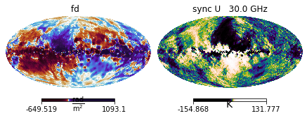
dset_fd = img_data.HEALPix.fd.Oppermann2012(Nside=32)
dset_sync = img_data.HEALPix.sync.Planck2018_Commander_U(Nside=32)
# Initialises ObservableDict objects
measurements = img.observables.Measurements(dset_fd, dset_sync)
# Shows the contents
measurements.show()
Observable names
Each type of observable has an agreed/conventional name. The presently available observable names are:
- Observable names
‘fd’ - Faraday depth
‘dm’ - Dispersion measure
‘sync’ - Synchrotron emission
- with tag ‘I’ - Total intensity
- with tag ‘Q’ - Stokes Q
- with tag ‘U’ - Stokes U
- with tag ‘PI’ - polarisation intensity
- with tag ‘PA’ - polarisation angle
Tabular datasets
As the name indicates, in tabular datasets the observational data was originally in tabular format, i.e. a table where each row corresponds to a different position in the sky and columns contain (at least) the sky coordinates, the measurement and the associated error. A final requirement is that the dataset is stored in a dictionary-like object i.e. the columns can be selected by column name (for example, a Python dictionary, a Pandas DataFrame, or an astropy Table).
To construct a tabular dataset, one needs to initialize
imagine.observables.TabularDataset.
Below, a simple example of this, which fetches (using the package astroquery)
a catalog from ViZieR and stores in in an IMAGINE tabular dataset object:
from astroquery.vizier import Vizier
from imagine.observables import TabularDataset

# Fetches the catalogue
catalog = Vizier.get_catalogs('J/ApJ/714/1170')[0]

# Loads it to the TabularDataset (the catalogue obj actually contains units)
RM_Mao2010 = TabularDataset(catalog, name='fd', units=catalog['RM'].unit,
                            data_col='RM', err_col='e_RM', tag=None,
                            lat_col='GLAT', lon_col='GLON')
From this point the object RM_Mao2010 can be appended to a
Measurements.
We refer the reader to the
the Including new observational data tutorial
and the
TabularDataset api
documentation and for further details.
HEALPix datasets
HEALPix datasets will generally comprise maps of the full-sky, where
HEALPix pixelation is employed.
For standard observables, the datasets can be initialized by simply supplying
a Quantity array containing the data to the
corresponding class. Below some examples, employing
the classes
FaradayDepthHEALPixDataset,
DispersionMeasureHEALPixDataset and
SynchrotronHEALPixDataset,
respectively:
from imagine.observables import FaradayDepthHEALPixDataset
from imagine.observables import DispersionMeasureHEALPixDataset
from imagine.observables import SynchrotronHEALPixDataset

my_FD_dset = FaradayDepthHEALPixDataset(data=fd_data_array,
                                        error=fd_data_array_error)

my_DM_dset = DispersionMeasureHEALPixDataset(data=fd_data_array,
                                             cov=fd_data_array_covariance)

sync_dset = SynchrotronHEALPixDataset(data=stoke_Q_data,
                                      error=stoke_Q_data_error
                                      frequency=23*u.GHz, type='Q')
In the first and third examples, it was assumed that the covariance was diagonal, and therefore can be described by an error associated with each pixel, which is specified with the keyword argument error (the error is assumed to correspond to the square root of the variance in each datapoint).
In the second example, the covariance associated with the data is instead specified supplying a two-dimensional array using the the cov keyword argument.
The final example also requires the user to supply the frequency of the observation and the subtype (in this case, ‘Q’).
Observables and observable dictionaries
In IMAGINE, observable quantities (either measured or simulated) are
represented internally by instances of the
imagine.observables.Observable
class. These are grouped in observable dictionaries (subclasses of
imagine.observables.ObservableDict)
which are used to exchange multiple observables between IMAGINE’s components.
There three main kinds of observable dictionaries: Measurements,
Simulations, and Covariances.
There is also an auxiliary observable dictionary: the Masks.
Measurements
The
imagine.observables.Measurements
object is used, as the name implies, to hold a set of actual measured physical
datasets (e.g. a set of intensity maps of the sky at different wavelengths).
A Measurements
object must be provided to initialize Simulators (allowing them to know
which datasets need to be computed) and Likelihoods.
There are a number of ways data can be provided to
Measurements.
The simplest case is when the data is stored in a Datasets objects, one can provide them to the
measurements object upon initialization:
measurements = img.observables.Measurements(dset1, dset2, dset3)
One can also append a dateset to a already initialized Measurements object:
measurements.append(dataset=dset4)
The final (not usually recommended) option is appending the data manually to the ObservableDict, which can be done in the following way:
measurements.append(name=key, data=data,
                    cov_data=cov, otype='HEALPix')
In this, data should contain a ndarray
or Quantity, cov_data should
contain the covariance matrix, and otype must indicate whether
the data corresponds to: a ‘HEALPix’ map; ‘tabular’; or a ‘plain’ array.
The name argument refers to the key that will be used to hash the
elements in the dictionary. This has to have the following form:
key = (data_name, data_freq, Nside_or_str, tag)
- The first value should be the one of the observable names
- If data is independent from frequency,
data_freqis set toNone, otherwise it is the frequency in GHz. - The third value in the key-tuple should contain the HEALPix Nside (for maps) or the string ‘tab’ for tabular data.
- Finally, the last value, ext can be ‘I’, ‘Q’, ‘U’, ‘PI’, ‘PA’,
Noneor other customized tags depending on the nature of the observable.
The contents of a
Measurements
object can be accessed as a dictionary, using the keys with the above
structure:
observable = measurements[('sync', 30, 32, 'I')]
Assuming that this key is present, the observable object returned
by the above line will be an instance of the
Observable
class. The data contents and properties can be then accessed using its
properties/attributes, for example:
data_array = observable.global_data
data_units = observable.unit
Where the data_array will be a (1, N)-array.
Measurements,
support the show
method (exemplified in Repository datasets) which displays a summary of
the data in the
ObservableDict.
Simulations
The Simulations
object is the
ObservableDict
that is returned when one runs an IMAGINE Simulator.
If the model does not involve any stochastic fields (or if the ensemble size is chosen to be 1), the Simulations object produced by a simulator has exactly the same structure as Measurements object.
For larger ensemble sizes the behaviour is slightly different. The
global_data attribute will return an array of shape (N_ens, N),
containing one realisation per row. The
show
method will display the simulated results for the full ensemble, with one
realisation per row (this can be limited using max_realizations
keyword, which sets the maximum number of rows to be displayed).
Simulations objects provide two specialized convenience methods to
manipulate the simulated data in the case of ensemble_size>1. The
sub_sim
method allows one to construct a new Simulations object using only a subset
of the original ensemble (note that this can also be used prepare resamplings
for bootstrapping). The
estimate_covariances
method uses the finite ensemble in the Simulations object to estimate the
covariance matrices associated with each observable, which are returned as
Covariances object.
Covariances
imagine.observables.Covariances
are a special type of
ObservableDict
which stores the set of covariance matrices associated with set of observables.
Its behavour is similar to the
Measurements,
the main difference being that the global_data attribute returns a
(N,N) covariance matrix instead of (1,N)-array.
In practice, one rarely needs to initialize or work with an independent
Covariances object.
This is because a Covariances object is automatically generated when one
initializes a Measurements
a Dataset, and stored in the
Measurements object
cov attribute:
# The covariances associated with a measurements object
covariances = measurements.cov
When the original dataset only contained variance information (e.g. specified
using the error keyword when preparing a Dataset) the full covariance matrix is not
constructed on initialization. Instead, the variance alone is stored internally
and the covariance matrix construction is delayed until the first time the
properties global_data or data
are requested. If imagine.rc['distributed_arrays']
is set to True (not the default),
the covariance matrix is spread among the available MPI processes.
As many observational datasets are very large (i.e. very large N), and only
contain known variance information, it often unnecessary (or simply impractical)
to operate with full (sparse) covariance matrices. Instead, one can access
the variance stored in the Covariances object using the var
property:
# An Observable object containing covariance information for a given key
cov_observable = covariances[('sync', 30, 32, 'I')]
# Reads the N-array containing the variances
variances = cov_observable.var
# Reads the (N,N)-array containing the covariance matrix
# (constructing it, if necessary)
cov_matrix = cov_observable.global_data
Thus, when working with large datasets some care should be take when choosing
(or designining) the Likelihood
class which will manipulate the Covariances object: some of the likelihoods
(e.g. EnsembleLikelihoodDiagonal)
only access the var attribute, keeping the RAM memory usage under control
even in the case of very large maps, while others will try construct the full
covariance matrix, potentially leading out-of-memory errors.
Masks
imagine.observables.Masks
which stores masks which can be applied to HEALPix maps. The mask itself is
specified in the form of an array of zeros and ones.
Simulators
Simulators are reponsible for mapping a set of Fields onto a set of
Observables. They are represented by a subclass of
imagine.simulators.Simulator.
from imagine.simulators import Simulator
import numpy as np
import MY_SIMULATOR  # Substitute this by your own code

class SimulatorTemplate(Simulator):
    """
    Detailed description of the simulator
    """
    # The quantity that will be simulated (e.g. 'fd', 'sync', 'dm')
    # Any observable quantity absent in this list is ignored by the simulator
    SIMULATED_QUANTITIES = ['my_observable_quantity']
    # A list or set of what is required for the simulator to work
    REQUIRED_FIELD_TYPES = ['dummy', 'magnetic_field']
    # Fields which may be used if available
    OPTIONAL_FIELD_TYPES = ['thermal_electron_density']
    # One must specify which grid is compatible with this simulator
    ALLOWED_GRID_TYPES = ['cartesian']
    # Tells whether this simulator supports using different grids
    USE_COMMON_GRID = False

    def __init__(self, measurements, **extra_args):
        # Send the measurements to parent class
        super().__init__(measurements)
        # Any initialization task involving **extra_args can be done *here*
        pass

    def simulate(self, key, coords_dict, realization_id, output_units):
        """
        This is the main function you need to override to create your simulator.
        The simulator will cycle through a series of Measurements and create
        mock data using this `simulate` function for each of them.

        Parameters
        ----------
        key : tuple
            Information about the observable one is trying to simulate
        coords_dict : dictionary
            If the trying to simulate data associated with discrete positions
            in the sky, this dictionary contains arrays of coordinates.
        realization_id : int
            The index associated with the present realisation being computed.
        output_units : astropy.units.Unit
            The requested output units.
        """
        # The argument key provide extra information about the specific
        # measurement one is trying to simulate
        obs_quantity, freq_Ghz, Nside, tag = key

        # If the simulator is working on tabular data, the observed
        # coordinates can be accessed from coords_dict, e.g.
        lat, lon = coords_dict['lat'], coords_dict['lon']

        # Fields can be accessed from a dictionary stored in self.fields
        B_field_values = self.fields['magnetic_field']
        # If a dummy field is being used, instead of an actual realisation,
        # the parameters can be accessed from self.fields['dummy']
        my_dummy_field_parameters = self.fields['dummy']
        # Checklists allow _dummy fields_ to send specific information to
        # simulators about specific parameters
        checklist_params = self.field_checklist
        # Controllists in dummy fields contain a dict of simulator settings
        simulator_settings = self.controllist

        # If a USE_COMMON_GRID is set to True, the grid it can be accessed from
        # grid = self.grid

        # Otherwise, if fields are allowed to use different grids, one can
        # get the grid from the self.grids dictionary and the field type
        grid_B = self.grids['magnetic_field']

        # Finally we can _simulate_, using whichever information is needed
        # and your own MY_SIMULATOR code:
        results = MY_SIMULATOR.simulate(simulator_settings,
                                        grid_B.x, grid_B.y, grid_B.z,
                                        lat, lon, freq_Ghz, B_field_values,
                                        my_dummy_field_parameters,
                                        checklist_params)
        # The results should be in a 1-D array of size compatible with
        # your dataset. I.e. for tabular data: results.size = lat.size
        # (or any other coordinate)
        # and for HEALPix data  results.size = 12*(Nside**2)

        # Note: Awareness of other observables
        # While this method will be called for each individual observable
        # the other observables can be accessed from self.observables
        # Thus, if your simulator is capable of computing multiple observables
        # at the same time, the results can be saved to an attribute on the first
        # call of `simulate` and accessed from this cache later.
        # To break the degeneracy between multiple realisations (which will
        # request the same key), the realisation_id can be used
        # (see Hammurabi implementation for an example)
        return results
Likelihoods
Likelihoods define how to quantitatively compare the simulated and measured
observables. They are represented within IMAGINE by an instance of class
derived from
imagine.likelihoods.Likelihood.
There are two pre-implemented subclasses within IMAGINE:
imagine.likelihoods.SimpleLikelihood: this is the traditional method, which is like a \(\chi^2\) based on the covariance matrix of the measurements (i.e., noise).imagine.likelihoods.EnsembleLikelihood: combines covariance matrices from measurements with the expected galactic variance from models that include a stochastic component.
Likelihoods need to be initialized before running the pipeline, and require measurements (at the front end). In most cases, data sets will not have covariance matrices but only noise values, in which case the covariance matrix is only the diagonal.
from imagine.likelihoods import EnsembleLikelihood
likelihood = EnsembleLikelihood(data, covariance_matrix)
The optional input argument covariance_matrix does not have to contain covariance matrices corresponding to all entries in input data. The Likelihood automatically defines the proper way for the various cases.
If the
EnsembleLikelihood
is used, then the sampler will be run multiple times at each point in likelihood space to create an ensemble of simulated observables.
Priors
A powerful aspect of a fully Baysean analysis approach is the possibility of
explicitly stating any prior expectations about the parameter values based on
previous knowledge. A prior is represented by an instance of
imagine.priors.prior.GeneralPrior or one of its subclasses.
To use a prior, one has to initialize it and include it in the associated
Field Factories. The simplest choice is a FlatPrior
(i.e. any parameter within the range are equally likely before the looking at
the observational data), which can be initialized in the following way:
from imagine.priors import FlatPrior
import astropy.units as u
myFlatPrior = FlatPrior(interval=[-2,10]*u.pc)
where the range for this parameter was chosen to be between \(-2\) and \(10\rm pc\).
After the flat prior, a common choice is that the parameter values are
characterized by a Gaussian distribution around some central value.
This can be achieved using the
imagine.priors.basic_priors.GaussianPrior class. As an example,
let us suppose one has a parameter which characterizes the strength of a
component of the magnetic field, and that ones prior expectation is that this
should be gaussian distributed with mean \(1\mu\rm G\) and standard
deviation \(5\mu\rm G\). Moreover, let us assumed that the model only works
within the range \([-30\mu \rm G, 30\mu G]\). A prior consistent with these
requirements can be achieved using:
from imagine.priors import GaussianPrior
import astropy.units as u
myGaussianPrior = GaussianPrior(mu=1*u.microgauss, sigma=5*u.microgauss,
                                interval=[-30*u.microgauss,30*u.microgauss])
Pipeline
The final building block of an IMAGINE pipeline is the Pipline object. When working on a problem with IMAGINE one will always go through the following steps:
1. preparing a list of the field factories which define the theoretical models one wishes to constrain and specifying any priors;
2. preparing a measurements dictionary, with the observational data to be used for the inference; and
3. initializing a likelihood object, which defines how the likelihood function should be estimated;
once this is done, one can supply all these to a Pipeline object, which will sample the posterior distribution and estimate the evidence. This can be done in the following way:
from imagine.pipelines import UltranestPipeline
# Initialises the pipeline
pipeline = UltranestPipeline(simulator=my_simulator,
                                 factory_list=my_factory_list,
                                 likelihood=my_likelihood,
                                 ensemble_size=my_ensemble_size_choice)
# Runs the pipeline
pipeline()
After running, the results can be accessed through the attributes of the
Pipeline object (e.g.
pipeline.samples,
which contains the parameters values of the samples produced in the run).
But what exactly is the Pipeline? The
Pipeline base class takes
care of interfacing between all the different IMAGINE components and sets the
scene so that a Monte Carlo sampler can explore the parameter space and
compute the results (i.e. posterior and evidence).
Different samplers are implemented as sub-classes of the Pipeline
There are 3 samplers included in IMAGINE standard distribution (alternatives
can be found in some of the
IMAGINE Consortium repositories),
these are: the MultinestPipeline,
the UltranestPipeline and the DynestyPipeline.
One can include a new sampler in IMAGINE by creating a sub-class of
imagine.Pipeline.
The following template illustrates this procedure:
from imagine.pipelines import Pipeline
import numpy as np
import MY_SAMPLER  # Substitute this by your own code

class PipelineTemplate(Pipeline):
    """
    Detailed description of sampler being adopted
    """
    # Class attributes
    # Does this sampler support MPI? Only necessary if True
    SUPPORTS_MPI = False

    def call(self, **kwargs):
        """
        Runs the IMAGINE pipeline

        Returns
        -------
        results : dict
            A dictionary containing the sampler results
            (usually in its native format)
        """
        # Initializes a sampler object
        # Here we provide a list of common options
        self.sampler = MY_SAMPLER.Sampler(
            # Active parameter names can be obtained from
            param_names=self.active_parameters,
            # The likelihood function is available in
            loglike=self._likelihood_function,
            # Some samplers need a "prior transform function"
            prior_transform=self.prior_transform,
            # Other samplers need the prior PDF, which is
            prior_pdf=self.prior_pdf,
            # Sets the directory where the sampler writes the chains
            chains_dir=self.chains_directory,
            # Sets the seed used by the sampler
            seed=self.master_seed
            )

        # Most samplers have a `run` method, which should be executed
        self.sampling_controllers.update(kwargs)
        self.results = self.sampler.run(**self.sampling_controllers)

        # The samples should be converted to a numpy array and saved
        # to self._samples_array. This should have different samples
        # on different rows and each column corresponds to an active
        # parameter
        self._samples_array = self.results['samples']
        # The log of the computed evidence and its error estimate
        # should also be stored in the following way
        self._evidence = self.results['logz']
        self._evidence_err = self.results['logzerr']

        return self.results


    def get_intermediate_results(self):
        # If the sampler saves intermediate results on disk or internally,
        # these should be read here, so that a progress report can be produced
        # every `pipeline.n_evals_report` likelihood evaluations.
        # For this to work, the following should be added to the
        # `intermediate_results` dictionary (currently commented out):

        ## Sets current rejected/dead points, as a numpy array of shape (n, npar)
        #self.intermediate_results['rejected_points'] = rejected
        ## Sets likelihood value of *rejected* points
        #self.intermediate_results['logLikelihood'] = likelihood_rejected
        ## Sets the prior volume/mass associated with each rejected point
        #self.intermediate_results['lnX'] = rejected_data[:, nPar+1]
        ## Sets current live nested sampling points (optional)
        #self.intermediate_results['live_points'] = live

        pass
Disclaimer
Nothing is written in stone and the base classes may be updated with time (so, always remember to report the code release when you make use of IMAGINE). Suggestions and improvements are welcome as GitHub issues or pull requests