Fields and Factories
Within the IMAGINE pipeline, spatially varying physical quantities are represented by Field objects. This can be a scalar, as the number density of thermal electrons, or a vector, as the Galactic magnetic field.
In order to extend or personalise adding in one’s own model for an specific field, one needs to follow a small number of simple steps:
- choose a coordinate grid where your model will be evaluated,
- write a field class, and
- write a field factory class.
The field objects will do the actual computation of the physical field, given a set of physical parameters and a coordinate grid. The field factory objects take care of book-keeping tasks: e.g. they hold the parameter ranges and default values, and translate the dimensionless parameters used by the sampler (always in the interval \([0,1]\)) to physical parameters, and hold the prior information on the parameter values.
Coordinate grid
You can create your own coordinate grid by subclassing imagine.fields.grid.BaseGrid. The only thing which has to actually be programmed in the new sub-class is a method overriding generate_coordinates(), which produces a dictionary of numpy arrays containing coordinates in either cartesian, cylindrical or spherical coordinates (generally assumed, in Galactic contexts, to be centred in the centre of the Milky Way).
Typically, however, it is sufficient to use a simple grid with coordinates uniformly-spaced in cartesian, spherical or cylindrical coordinates. This can be done using the UniformGrid class. UniformGrid objects are initialized with the arguments: box, which contains the ranges of each coordinate in \(\rm kpc\) or \(\rm rad\); resolution, a list of integers containing the number of grid points on each dimension; and grid_type, which can be either ‘cartesian’ (default),
‘cylindrical’ or ‘spherical’.
[1]:
import imagine as img
import numpy as np
import astropy.units as u
# Fixes numpy seed to ensure this notebook leads always to the same results
np.random.seed(42)

# A cartesian grid can be constructed as follows
cartesian_grid = img.fields.UniformGrid(box=[[-15*u.kpc, 15*u.kpc],
                                             [-15*u.kpc, 15*u.kpc],
                                             [-15*u.kpc, 15*u.kpc]],
                                        resolution = [15,15,15])

# For cylindrical grid, the limits are specified assuming
# the order: r (cylindrical), phi, z
cylindrical_grid = img.fields.UniformGrid(box=[[0.25*u.kpc, 15*u.kpc],
                                               [-180*u.deg, np.pi*u.rad],
                                               [-15*u.kpc, 15*u.kpc]],
                                          resolution = [9,12,9],
                                          grid_type = 'cylindrical')

# For spherical grid, the limits are specified assuming
# the order: r (spherical), theta, phi (azimuth)
spherical_grid = img.fields.UniformGrid(box=[[0*u.kpc, 15*u.kpc],
                                             [0*u.rad, np.pi*u.rad],
                                             [-np.pi*u.rad,np.pi*u.rad]],
                                        resolution = [12,10,10],
                                        grid_type = 'spherical')
The grid object will produce the grid only when the a coordinate value is first accessed, through the properties ‘x’, ‘y’,’z’,’r_cylindrical’,’r_spherical’, ‘theta’ and ‘phi’.
The grid object also takes care of any coordinate conversions that are needed, for example:
[2]:
print(spherical_grid.x[5,5,5], cartesian_grid.r_spherical[5,5,5])
6.309658489079476 kpc 7.423074889580904 kpc
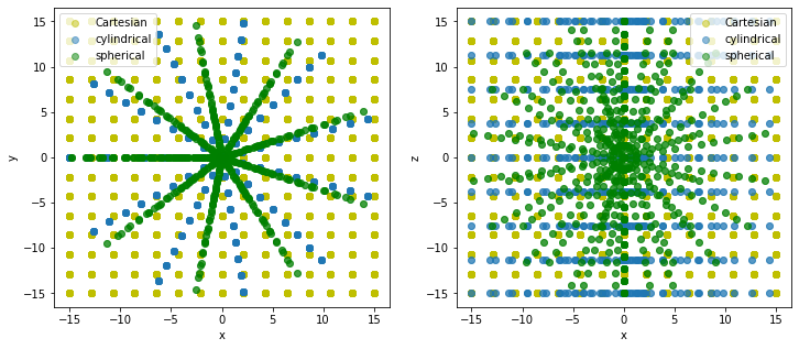
In the following figure we illustrate the effects of different choices of ‘grid_type’ while using UniformGrid.
(Note that, for plotting purposes, everything is converted to cartesian coordinates)
[3]:
import matplotlib.pyplot as plt

plt.figure(figsize=(12,5))
plt.subplot(1,2,1)
plt.scatter(cartesian_grid.x, cartesian_grid.y, color='y', label='Cartesian', alpha=0.5)
plt.scatter(cylindrical_grid.x, cylindrical_grid.y, label='cylindrical', alpha=0.5)
plt.scatter(spherical_grid.x, spherical_grid.y, color='g', label='spherical', alpha=0.5)
plt.xlabel('x'); plt.ylabel('y')
plt.legend()

plt.subplot(1,2,2)
plt.scatter(cartesian_grid.x, cartesian_grid.z, color='y', label='Cartesian', alpha=0.5)
plt.scatter(cylindrical_grid.x, cylindrical_grid.z, label='cylindrical', alpha=0.5)
plt.scatter(spherical_grid.x, spherical_grid.z, label='spherical', color='g', alpha=0.5)
plt.xlabel('x'); plt.ylabel('z')
plt.legend();
Field objects
As we mentioned before, Field objects handle the calculation of any physical field.
To ensure that your new personalised field is compatible with any simulator, it needs to be a subclass of one of the pre-defined field classes. Some examples of which are:
MagneticFieldThermalElectronDensityCosmicRayDistribution
Let us illustrate this by defining a thermal electron number density field which decays exponentially with cylindrical radius, \(R\),
This has three parameters: the number density of thermal electrons at the centre, \(n_{e,0}\), the scale radius, \(R_e\), and the scale height, \(h_e\).
[4]:
from imagine.fields import ThermalElectronDensityField

class ExponentialThermalElectrons(ThermalElectronDensityField):
    """Example: thermal electron density of an (double) exponential disc"""

    NAME = 'exponential_disc_thermal_electrons'
    PARAMETER_NAMES = ['central_density', 'scale_radius', 'scale_height']

    def compute_field(self, seed):
        R = self.grid.r_cylindrical
        z = self.grid.z
        Re = self.parameters['scale_radius']
        he = self.parameters['scale_height']
        n0 = self.parameters['central_density']

        return n0*np.exp(-R/Re)*np.exp(-np.abs(z/he))
With these few lines we have created our IMAGINE-compatible™ thermal electron density field class!
The class-attribute NAME allows one to keep track of which model we have used to generate our field.
The PARAMETER_NAMES attribute must contain all the required parameters for this particular kind of field.
The function compute_field is what actually computes the density field. Note that it can access an associated grid object, which is stored in the grid attribute, and a dictionary of parameters, stored in the parameters attribute. The compute_field method takes a seed argument, which can is only used for stochastic fields (see later).
Let us now see this at work. First, let us creat an instance of ExponentialThermalElectrons. Any Field instance should be initialized providing a Grid object and a dictionary of parameters.
[5]:
electron_distribution = ExponentialThermalElectrons(
    parameters={'central_density': 1.0*u.cm**-3,
                'scale_radius': 3.3*u.kpc,
                'scale_height': 3.3*u.kpc},
    grid=cartesian_grid)
We can access the field produced by cr_distribution using the get_data() method (it invokes compute_field internally and does any checking required). For example:
[6]:
ne_data = electron_distribution.get_data()
print('data is', type(ne_data), 'of length', ne_data.shape)
print('an example slice of it is:')
ne_data[3:5,3:5,3:5]
data is <class 'astropy.units.quantity.Quantity'> of length (15, 15, 15)
an example slice of it is:
[6]:
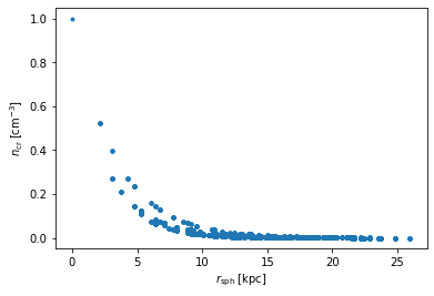
If we now wanted to plot the thermal electron density computed by this as a function of, say, spherical radius, \(r_{\rm sph}\). This can be done in the following way
[7]:
# The spherical radius can be read from the grid object
rspherical = electron_distribution.grid.r_spherical

plt.plot(rspherical.ravel(), ne_data.ravel(), '.')
plt.xlabel(r'$r_{\rm sph}\;[\rm kpc]$'); plt.ylabel(r'$n_{\rm cr}\;[\rm cm^{-3}]$');
Let us do another simple field example: a constant magnetic field.
It follows the same basic template.
[8]:
from imagine.fields import MagneticField

class ConstantMagneticField(MagneticField):
    """Example: constant magnetic field"""
    NAME = 'constantB'
    PARAMETER_NAMES = ['Bx', 'By', 'Bz']

    def compute_field(self, seed):
        # Creates an empty array to store the result
        B = np.empty(self.data_shape) * self.parameters['Bx'].unit
        # For a magnetic field, the output must be of shape:
        # (Nx,Ny,Nz,Nc) where Nc is the index of the component.
        # Computes Bx
        B[:,:,:,0] = self.parameters['Bx']*np.ones(self.grid.shape)
        # Computes By
        B[:,:,:,1] = self.parameters['By']*np.ones(self.grid.shape)
        # Computes Bz
        B[:,:,:,2] = self.parameters['Bz']*np.ones(self.grid.shape)
        return B
The main difference from the thermal electrons case is that the shape of the final array has to accomodate all the three components of the magnetic field.
As before, we can generate a realisation of this
[9]:
p = {'Bx': 1.5*u.microgauss, 'By': 1e-10*u.Tesla, 'Bz': 0.1e-6*u.gauss}
B = ConstantMagneticField(parameters=p, grid=cartesian_grid)
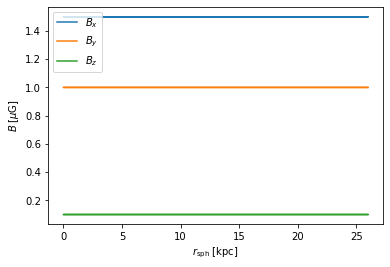
And inspect how it went
[10]:
r_spherical = B.grid.r_spherical.ravel()
B_data = B.get_data()
for i, name in enumerate(['x','y','z']):
    plt.plot(r_spherical, B_data[...,i].ravel(),
             label='$B_{}$'.format(name))
plt.xlabel(r'$r_{\rm sph}\;[\rm kpc]$'); plt.ylabel(r'$B\;[\mu\rm G]$')
plt.legend();
More information about the field can be found inspecting the object
[11]:
print('Field type: ', B.type)
print('Data shape: ', B.data_shape)
print('Units: ', B.units)
print('What is each axis? Answer:', B.data_description)
Field type:  magnetic_field
Data shape:  (15, 15, 15, 3)
Units:  uG
What is each axis? Answer: ['grid_x', 'grid_y', 'grid_z', 'component (x,y,z)']
Let us now exemplify the construction of a stochastic field with a thermal electron density comprising random fluctuations.
[12]:
from imagine.fields import ThermalElectronDensityField
import scipy.stats as stats

class RandomThermalElectrons(ThermalElectronDensityField):
    """Example: Gaussian random thermal electron density

    NB this may lead to negative ne depending on the choice of
    parameters.
    """

    NAME = 'random_thermal_electrons'
    STOCHASTIC_FIELD = True
    PARAMETER_NAMES = ['mean', 'std']

    def compute_field(self, seed):
        # Converts dimensional parameters into numerical values
        # in the correct units
        mu = self.parameters['mean'].to_value(self.units)
        sigma = self.parameters['std'].to_value(self.units)
        # Draws values from a normal distribution with these parameters
        # using the seed provided in the argument
        distr = stats.norm(loc=mu, scale=sigma)
        result = distr.rvs(size=self.data_shape, random_state=seed)

        return result*self.units # Restores units
The STOCHASTIC_FIELD class-attribute tells whether the field is deterministic (i.e. the output depends only on the parameter values) or stochastic (i.e. the ouput is a random realisation which depends on a particular random seed). If this is absent, IMAGINE assumes the field is deterministic.
In the example above, the field at each point of the grid is drawn from a Gaussian distribution described by the parameters ‘mean’ and ‘std’, and the seed argument is used to initialize the random number generator.
[13]:
rnd_electron_distribution = RandomThermalElectrons(
    parameters={'mean': 1.0*u.cm**-3,
                'std': 0.25*u.cm**-3},
    grid=cartesian_grid, ensemble_size=4)
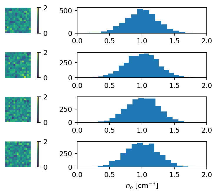
The previous code generates an ensemble with 4 realisations of the random field. In order to inspect it, let us plot, for each realisation, a slice of the thermal electron density, and a histogram of \(n_e\). Again, we can use the get_data method, but this time we provide the index of each realisation.
[14]:
j = 0; plt.figure(dpi=170)
for i in range(4):
    rnd_e_data = rnd_electron_distribution.get_data(i_realization=i
                                      )
    j += 1; plt.subplot(4,2,j)

    plt.imshow(rnd_e_data[0,:,:].value, vmin=0, vmax=2)
    plt.axis('off')
    plt.colorbar()
    j += 1; plt.subplot(4,2,j)
    plt.hist(rnd_e_data.value.ravel(), bins=20)
    plt.xlim(0,2)
plt.xlabel(r'$n_e\; \left[ \rm cm^{-3}\right] $');
plt.tight_layout()
The previous results were generated for the randomly chosen random seeds:
[15]:
rnd_electron_distribution.ensemble_seeds
[15]:
array([1935803228, 787846414, 996406378, 1201263687])
Alternatively, to ensure reproducibility, one can explicitly provide the seeds instead of the ensemble size.
[16]:
rnd_electron_distribution = RandomThermalElectrons(
        parameters={'mean': 1.0*u.cm**-3,
                'std': 0.25*u.cm**-3},
    grid=cartesian_grid, ensemble_seeds=[11,22,33,44])

rnd_electron_distribution.ensemble_size, rnd_electron_distribution.ensemble_seeds
[16]:
(4, [11, 22, 33, 44])
Before moving on, there is one specialised field type which is worth mentioning: the dummy field.
Dummy fields are used when one wants to send (varying) parameters directly to the simulator, i.e. this Field object does not evaluate anything but the pipeline is still able to vary its parameters.
Why would anyone want to do this? First of all, it is worth remembering that, within the Bayesian framework, the “model” is the Field together with the Simulator, and the latter can also be parametrised. In other words, there can be parameters which control how to convert a set of models for physical fields into observables.
Another possibility is that a specific Simulator (e.g. Hammurabi) already contains built-in parametrised fields which one is willing to make use of. Dummy fields allow one to vary those parameters easily.
compute_field,STOCHASTIC_FIELD or PARAMETER_NAMES).[17]:
from imagine.fields import DummyField

class exampleDummy(DummyField):
    NAME = 'example_dummy'
    FIELD_CHECKLIST = {'A': None, 'B': 'foo', 'C': 'bar'}
    SIMULATOR_CONTROLLIST = {'lookup_directory': '/dummy/example',
                             'choice_of_settings': ['tutorial','field']}
Thus, instead of a PARAMETER_NAMES, one needs to specify a FIELD_CHECKLIST which contains a dictionary with parameter names as keys. Its main use is to send to the Simulator fixed settings associated with a particular parameter. For example, the FIELD_CHECKLIST is used by the Hammurabi-compatible dummy fields to inform the Simulator class where in Hammurabi XML file the parameter value should be saved.
The extra SIMULATOR_CONTROLLIST attribute plays a similar role: it is used to send settings associated with a field which are not associated with individual model parameters to the Simulator. A typical use is the setup of global switches which enable specific builtin field in
[18]:
dummy = exampleDummy(parameters={'A': 42,
                                 'B': 17*u.kpc,
                                 'C': np.pi},
                     ensemble_size=4)
That is it. Let us inspect the data associated with this Field:
[19]:
for i in range(4):
    print(dummy.get_data(i))
{'A': 42, 'B': <Quantity 17. kpc>, 'C': 3.141592653589793, 'random_seed': 423734972}
{'A': 42, 'B': <Quantity 17. kpc>, 'C': 3.141592653589793, 'random_seed': 415968276}
{'A': 42, 'B': <Quantity 17. kpc>, 'C': 3.141592653589793, 'random_seed': 670094950}
{'A': 42, 'B': <Quantity 17. kpc>, 'C': 3.141592653589793, 'random_seed': 1914837113}
Therefore, instead of actual data arrays, the get_data of a dummy field returns a copy of its parameters dictionary, supplemented by a random seed which can optionally be used by the Simulator to generate stochastic fields internally.
Field factory
Associated with each Field class we need to prepare a FieldFactory object, which, for each parameter, stores ranges, default values and priors.
This is done using the imagine.fields.FieldFactory class.
[20]:
from imagine.priors import FlatPrior

exp_te_factory = img.fields.FieldFactory(
    field_class=ExponentialThermalElectrons,
    grid=cartesian_grid,
    active_parameters=[],
    default_parameters = {'central_density': 1*u.cm**-3,
                          'scale_radius': 3.0*u.kpc,
                          'scale_height': 0.5*u.kpc})
[21]:
Bfactory = img.fields.FieldFactory(
    field_class=ConstantMagneticField,
    grid=cartesian_grid,
    active_parameters=['Bx'],
    default_parameters={'By': 5.0*u.microgauss,
                        'Bz': 0.0*u.microgauss},
    priors={'Bx': FlatPrior(xmin=-30*u.microgauss, xmax=30*u.microgauss)})
We can now create instances of any of these. The priors, defaults and also parameter ranges can be accessed using the related properties:
[22]:
Bfactory.default_parameters, Bfactory.parameter_ranges, Bfactory.priors
[22]:
({'By': <Quantity 5. uG>, 'Bz': <Quantity 0. uG>},
 {'Bx': <Quantity [-30.,  30.] uG>},
 {'Bx': <imagine.priors.basic_priors.FlatPrior at 0x7fb3b533da90>})
As a user, this is all there is to know about FieldFactories: one need to intialized them with the ones selection of active parameters, priors and default values and provide the initialized objects to the IMAGINE Pipeline class.
Internally, these instances can return Field objects (hence the name) when they are called internally by the Pipeline whilst running. This is exemplified below:
[23]:
newB = Bfactory(variables={'Bx': 0.9*u.microgauss})
print('field name: {}\nparameters: {}'.format(newB.name, newB.parameters))
field name: constantB
parameters: {'By': <Quantity 5. uG>, 'Bz': <Quantity 0. uG>, 'Bx': <Quantity 0.9 uG>}
In the previous definitions, a flat (i.e. uniform) prior was assumed for all the parameters. Setting up a personalised prior is discussed in detail in the Priors section below. Here we demonstrate how to setup a Gaussian prior for the parameters By and Bz, truncated in the latter case. The priors can be included creating an object GaussianPrior for which the mean, standard deviation and range are specified:
[24]:
from imagine.priors import GaussianPrior

muG = u.microgauss

Bfactory = img.fields.FieldFactory(
    field_class=ConstantMagneticField,
    grid=cartesian_grid,
    active_parameters=['Bx', 'By','Bz'],
    priors={'Bx': FlatPrior(xmin=-30*muG, xmax=30*muG),
            'By': GaussianPrior(mu=5*muG, sigma=10*muG),
            'Bz': GaussianPrior(mu=0*muG, sigma=3*muG,
                                xmin=-30*muG, xmax=30*muG)})
Let us now inspect an instance of updated field factory
[25]:
Bfactory.priors, Bfactory.parameter_ranges
[25]:
({'Bx': <imagine.priors.basic_priors.FlatPrior at 0x7fb3b532cc90>,
  'By': <imagine.priors.basic_priors.GaussianPrior at 0x7fb3b533db10>,
  'Bz': <imagine.priors.basic_priors.GaussianPrior at 0x7fb3b5329f50>},
 {'Bx': <Quantity [-30.,  30.] uG>,
  'By': <Quantity [-inf,  inf] uG>,
  'Bz': <Quantity [-30.,  30.] uG>})
We can visualise the selected priors through auxiliary methods in the objects. E.g.
[26]:
b = np.linspace(-30,30,100)*muG
plt.plot(b, Bfactory.priors['Bx'].pdf(b))
plt.plot(b, Bfactory.priors['By'].pdf(b))
plt.plot(b, Bfactory.priors['Bz'].pdf(b));
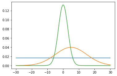
More details on how to define personalised priors can be found in the dedicated tutorial.
One final comment: the generate method can take the arguments ensemble_seeds or ensemble_size methods, propagating them to the fields it produces.
Dependencies between Fields
Sometimes, one may want to include in the inference a dependence between different fields (e.g. the cosmic ray distribution may depend on the underlying magnetic field, or the magnetic field may depend on the gas distribution). The IMAGINE can handle this (to a certain extent). In this section, we discuss how this works.
(NB This section is somewhat more advanced and we advice to skip it if this is your first contact with the IMAGINE software.)
Dependence on a field type
The most common case of dependence is when a particular model, expressed as a IMAGINE Field, depends on a ‘field type’, but not on another specific Field object - in other words: there is a dependence of one physical field on another physical field, and not a dependence of a particular model on another model). This is the case we are showing here.
As a concrete example, let us consider a (very artificial) model where \(y\)-component of the magnetic field strength is (for whatever reason) proportional to energy equipartition value. The Field object that represents such a field will, therefore, depend on the density distribution (which is is computed before, independently). The following snippet show how to code this.
[27]:
import astropy.constants as c
# unfortunatelly, astropy units does not perform the following automatically
gauss_conversion = u.gauss/(np.sqrt(1*u.g/u.cm**3)*u.cm/u.s)

class DependentBFieldExample(MagneticField):
    """Example: By depends on ne"""
    # Class attributes
    NAME = 'By_Beq'
    DEPENDENCIES_LIST = ['thermal_electron_density']
    PARAMETER_NAMES = ['v0']

    def compute_field(self, seed):
        # Gets the thermal electron number density from another Field
        te_density = self.dependencies['thermal_electron_density']

        # Computes the density, assuming electrons come from H atoms
        rho = te_density * c.m_p
        Beq = np.sqrt(4*np.pi*rho)*self.parameters['v0'] * gauss_conversion

        # Sets B
        B = np.zeros(self.data_shape) * u.microgauss
        B[:,:,:,1] = Beq

        return B
If there is a field type string in dependencies_list, the pipeline will, at run-time, automatically feed a dictionary in the attribute DependentBFieldExample.dependencies with the request. Thus, during a run of the Pipeline or a Simulator, the variable te_density will contain the sum of all ‘thermal_electron_density’ Field objects that had been supplied.
If we are willing to test the DependentBFieldExample above defined, we need to provide this ourselves. The following lines illustrate this.
[28]:
# Creates an instance
dependent_field = DependentBFieldExample(cartesian_grid,
                                         parameters={'v0': 10*u.km/u.s})

dependent_field_data = dependent_field.get_data(i_realization=0,
    dependencies={'thermal_electron_density': electron_distribution.get_data(i_realization=0)})

for i, name in enumerate(['x','y','z']):
    plt.plot(dependent_field.grid.r_cylindrical.ravel(),
             dependent_field_data[...,i].ravel(), '.',
             label='$B_{}$'.format(name))
plt.xlabel(r'$r_{\rm cyl}\;[\rm kpc]$'); plt.ylabel(r'$B\;[\mu\rm G]$')
plt.legend();
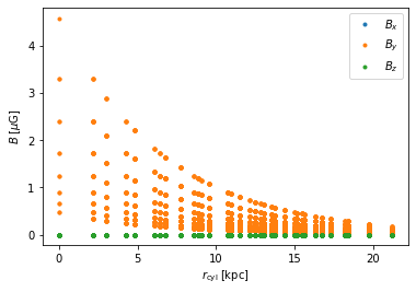
Thus, we see that \(B_y\) decays exponentially, tracking \(n_e\), and \(B_x=B_y=0\), as expected.
Note that, since this is a deterministic field, the i_realization argument may be suppressed. However, in the stochastic case, the realization index of the field and its dependencies must be aligned. (Again, this is only relevant for testing. When the Field is supplied to a Simulator, all this book-keeping is handled automatically).
Dependence on a field class
The second case is when a specific Field object depends on another Field object.
There are many situations where this may be needed, perhaps the most common two are:
- we have two or more Fields which share some parameters;
- we would like to write a wrapper Field classes for some pre-existing code that computes two or more physical fields at the same time.
For the latter case, the behaviour we would like to have is the following: when the first Field is invoked, the results must to be temporarily saved and later accessd by the others.
The following code illustrated the syntax to achieve this.
[29]:
class ConstantElectrons(ThermalElectronDensityField):
    NAME = 'constant_thermal_electron_density'
    PARAMETER_NAMES = ['A']

    def compute_field(self, seed):
        #
        ne = np.ones(self.data_shape) << u.cm**-3
        ne *= self.parameters['A']
        # Suppose together with the previous calculation
        # we had computed a component of B, we can save
        # this information as an attribute
        self.Bz_should_be = 17*u.microgauss
        return  ne


class ConstantDependentB(MagneticField):
    """Example: constant magnetic field dependent on ConstantElectrons"""
    NAME = 'constantBdep'
    DEPENDENCIES_LIST = [ConstantElectrons]
    PARAMETER_NAMES = []

    def compute_field(self, seed):

        # Gets the instance of the requested ConstantElectrons class
        ConstantElectrons_object = self.dependencies[ConstantElectrons]

        # Reads the common parameter A
        A = ConstantElectrons_object.parameters['A']

        # Initializes the B-field
        B = np.ones(self.data_shape) * u.microgauss
        # Sets Bx and By using A
        B[:,:,:,:2] *= np.sqrt(A)

        # Uses a Bz tha was computed earlier, elsewhere!
        B[:,:,:,2] = ConstantElectrons_object.Bz_should_be

        return B
If a ‘class’ is provided in the dependency list, the simulator will populate the dependencies attribute with the key-value pair: (FieldClass: FieldObject), where the FieldObject had been evaluated earlier.
If we are willing to test, we can feed the dependencies ourselves in the following way.
[30]:
# Initializes the instances
ne_field = ConstantElectrons(cartesian_grid, parameters={'A': 64})
dependent_field = ConstantDependentB(cartesian_grid)

# Evaluates the ne_field
ne_field_data = ne_field.get_data()
# Evaluates the dependent B_field
dependent_field_data = dependent_field.get_data(
        dependencies={ConstantElectrons: ne_field})
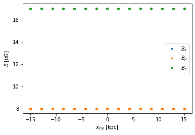
[31]:
for i, name in enumerate(['x','y','z']):
    plt.plot(dependent_field.grid.x.ravel(),
             dependent_field_data[...,i].ravel(), '.',
             label='$B_{}$'.format(name))
plt.xlabel(r'$x_{\rm cyl}\;[\rm kpc]$'); plt.ylabel(r'$B\;[\mu\rm G]$')
plt.legend();