Including new observational data
In this tutorial we will see how to load observational data onto IMAGINE.
Both observational and simulated data are manipulated within IMAGINE through observable dictionaries. There are three types of these: Measurements, Simulations and Covariances, which can store multiple entries of observational, simulated and covariance (either real or mock) data, respectively. Appending data to an ObservableDict requires following some requirements regarding the data format, therefore we recomend the use of one of the Dataset classes.
HEALPix Datasets
Let us illustrate how to prepare an IMAGINE dataset with the Faraday depth map obtained by Oppermann et al. 2012 (arXiv:1111.6186).
The following snippet will download the data (a ~4MB FITS file) to RAM and open it.
[1]:
import requests, io
from astropy.io import fits

download = requests.get('https://wwwmpa.mpa-garching.mpg.de/ift/faraday/2012/faraday.fits')
raw_dataset = fits.open(io.BytesIO(download.content))
raw_dataset.info()
Filename: <class '_io.BytesIO'>
No.    Name      Ver    Type      Cards   Dimensions   Format
  0  PRIMARY       1 PrimaryHDU       7   ()
  1  TEMPERATURE    1 BinTableHDU     17   196608R x 1C   [E]
  2  signal uncertainty    1 BinTableHDU     17   196608R x 1C   [E]
  3  Faraday depth    1 BinTableHDU     17   196608R x 1C   [E]
  4  Faraday uncertainty    1 BinTableHDU     17   196608R x 1C   [E]
  5  galactic profile    1 BinTableHDU     17   196608R x 1C   [E]
  6  angular power spectrum of signal    1 BinTableHDU     12   384R x 1C   [E]
Now we will feed this to an IMAGINE Dataset. It requires converting the data into a proper numpy array of floats. To allow this notebook running on a small memory laptop, we will also reduce the size of the arrays (only taking 1 value every 256).
[2]:
from imagine.observables import FaradayDepthHEALPixDataset
import numpy as np
from astropy import units as u
import healpy as hp

# Adjusts the data to the right format
fd_raw = raw_dataset[3].data.astype(np.float)
sigma_fd_raw = raw_dataset[4].data.astype(np.float)
# Makes it smaller, to save memory
fd_raw = hp.pixelfunc.ud_grade(fd_raw, 4)
sigma_fd_raw = hp.pixelfunc.ud_grade(sigma_fd_raw, 4)
# We need to include units the data
# (this avoids later errors and inconsistencies)
fd_raw *= u.rad/u.m/u.m
sigma_fd_raw *= u.rad/u.m/u.m
# Loads into a Dataset
dset = FaradayDepthHEALPixDataset(data=fd_raw, error=sigma_fd_raw)
One important assumption in the previous code-block is that the covariance matrix is diagonal, i.e. that the errors in FD are uncorrelated. If this is not the case, instead of initializing the FaradayDepthHEALPixDataset with data and error, one should initialize it with data and cov, where the latter is the correct covariance matrix.
To keep things organised and useful, we strongly recommend to create a personalised dataset class and make it available to the rest of the consortium in the imagine-datasets GitHub repository. An example of such a class is the following:
[3]:
from imagine.observables import FaradayDepthHEALPixDataset

class FaradayDepthOppermann2012(FaradayDepthHEALPixDataset):
    def __init__(self, Nside=None):
        # Fetches and reads the
        download = requests.get('https://wwwmpa.mpa-garching.mpg.de/ift/faraday/2012/faraday.fits')
        raw_dataset = fits.open(io.BytesIO(download.content))
        # Adjusts the data to the right format
        fd_raw = raw_dataset[3].data.astype(np.float)
        sigma_fd_raw = raw_dataset[4].data.astype(np.float)
        # Reduces the resolution
        if Nside is not None:
            fd_raw = hp.pixelfunc.ud_grade(fd_raw, Nside)
            sigma_fd_raw = hp.pixelfunc.ud_grade(sigma_fd_raw, Nside)
        # Includes units in the data
        fd_raw *= u.rad/u.m/u.m
        sigma_fd_raw *= u.rad/u.m/u.m
        # Loads into the Dataset
        super().__init__(data=fd_raw, error=sigma_fd_raw)
With this pre-programmed, anyone will be able to load this into the pipeline by simply doing
[4]:
dset = FaradayDepthOppermann2012(Nside=32)
In fact, this dataset is part of the imagine-datasets repository and can be immediately accessed using:
import imagine_datasets as img_data
dset = img_data.HEALPix.fd.Oppermann2012(Nside=32)
One of the advantages of using the datasets in the imagine_datasets repository is that they are cached to the hard disk and are only downloaded on the first time they are requested.
Now that we have a dataset, we can load this into a Measurements and Covariances objects (which will be discussed in detail further down).
[5]:
from imagine.observables import Measurements, Covariances

# Creates an instance
mea = Measurements()

# Appends the data
mea.append(dataset=dset)
If the dataset contains error or covariance data, its inclusion in a Measurements object automatically leads to the inclusion of such dataset in an associated Covariances object. This can be accessed through the cov attribute:
[6]:
mea.cov
[6]:
<imagine.observables.observable_dict.Covariances at 0x7ffaaf2f1d10>
An alternative, rather useful, supported syntax is providing the datasets as one initializes the Measurements object.
[7]:
# Creates _and_ appends
mea = Measurements(dset)
Tabular Datasets
So far, we looked into datasets comprising HEALPix maps. One may also want to work with tabular datasets. We exemplify this fetching and preparing a RM catalogue of Mao et al 2010 (arXiv:1003.4519). In the case of this particular dataset, we can import the data from VizieR using the astroquery library.
[8]:
import astroquery
from astroquery.vizier import Vizier

# Fetches the relevant catalogue from Vizier
# (see https://astroquery.readthedocs.io/en/latest/vizier/vizier.html for details)
catalog = Vizier.get_catalogs('J/ApJ/714/1170')[0]
catalog[:3] # Shows only first rows
[8]:
| RAJ2000 | DEJ2000 | GLON | GLAT | RM | e_RM | PI | I | S5.2 | f_S5.2 | NVSS |
|---|---|---|---|---|---|---|---|---|---|---|
| "h:m:s" | "d:m:s" | deg | deg | rad / m2 | rad / m2 | mJy | mJy | |||
| bytes11 | bytes11 | float32 | float32 | int16 | int16 | float32 | float64 | bytes3 | bytes1 | bytes4 |
| 13 07 08.33 | +24 47 00.7 | 0.21 | 85.76 | -3 | 4 | 7.77 | 131.49 | Yes | NVSS | |
| 13 35 48.14 | +20 10 16.0 | 0.86 | 77.70 | 3 | 5 | 8.72 | 71.47 | No | b | NVSS |
| 13 24 14.48 | +22 13 13.1 | 1.33 | 81.08 | -6 | 6 | 7.62 | 148.72 | Yes | NVSS |
The procedure for converting this to an IMAGINE data set is the following:
[9]:
from imagine.observables import TabularDataset
dset_tab = TabularDataset(catalog, name='fd', tag=None,
                          units= u.rad/u.m/u.m,
                          data_col='RM', err_col='e_RM',
                          lat_col='GLAT', lon_col='GLON')
catalog must be a dictionary-like object (e.g. dict, astropy.Tables, pandas.DataFrame) and data(/error/lat/lon)_column specify the key/column-name used to retrieve the relevant data from catalog. The name argument specifies the type of measurement that is being stored. This has to agree with the requirements of the Simulator you will use. Some standard available observable names are:
- ‘fd’ - Faraday depth
- ‘sync’ - Synchrotron emission, needs the
tagto be interpreted- tag = ‘I’ - Total intensity
- tag = ‘Q’ - Stokes Q
- tag = ‘U’ - Stokes U
- tag = ‘PI’ - polarisation intensity
- tag = ‘PA’ - polarisation angle
- ‘dm’ - Dispersion measure
The units are provided as an astropy.units.Unit object and are converted internally to the requirements of the specific Simulator being used.
Again, the procedure can be packed and distributed to the community in a (very short!) personalised class:
[10]:
from astroquery.vizier import Vizier
from imagine.observables import TabularDataset

class FaradayRotationMao2010(TabularDataset):
    def __init__(self):
        # Fetches the catalogue
        catalog = Vizier.get_catalogs('J/ApJ/714/1170')[0]
        # Reads it to the TabularDataset (the catalogue obj actually contains units)
        super().__init__(catalog, name='fd', units=catalog['RM'].unit,
                         data_col='RM', err_col='e_RM',
                         lat_col='GLAT', lon_col='GLON')
[11]:
dset_tab = FaradayRotationMao2010() # ta-da!
Measurements and Covariances
Again, we can include these observables in our Measurements object. This is a dictionary-like object, i.e. given a key, one can access a given item.
[12]:
mea.append(dataset=dset_tab)

print('Measurement keys:')
for k in mea.keys():
    print('\t',k)
Measurement keys:
         ('fd', None, 32, None)
         ('fd', None, 'tab', None)
Associated with the Measurements objects there is a Covariances object which stores the covariance matrix associated with each entry in the Measurements. This is also an ObservableDict subclass and has, therefore, similar behaviour. If the original Dataset contained error information but no full covariance data, a diagonal covariance matrix is assumed. (N.B. correlations between different observables – i.e. different entries in the Measurements object – are still not
supported.)
[13]:
print('Covariances dictionary', mea.cov)
print('\nCovariance keys:')
for k in mea.cov.keys():
    print('\t',k)
Covariances dictionary <imagine.observables.observable_dict.Covariances object at 0x7ffaaf00d750>

Covariance keys:
         ('fd', None, 32, None)
         ('fd', None, 'tab', None)
The keys follow a strict convention: (data-name,data-freq,Nside/'tab',ext)
- If data is independent from frequency, data-freq is set
None, otherwise it is the frequency in GHz. - The third value in the key-tuple is the HEALPix Nside (for maps) or the string ‘tab’ for tabular data.
- Finally, the last value,
extcan be ‘I’,’Q’,’U’,’PI’,’PA’, None or other customized tags depending on the nature of the observable.
Accessing and visualising data
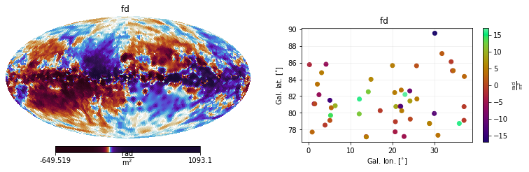
Frequently, one may want to see what is inside a given Measurements object. For this, one can use the handy helper method show(), which automatically displays all the contents of your Measurements object.
[14]:
import matplotlib.pyplot as plt
plt.figure(figsize=(12,3))

mea.show()
/home/lrodrigues/miniconda3/envs/imagine/lib/python3.7/site-packages/healpy/projaxes.py:209: MatplotlibDeprecationWarning: Passing parameters norm and vmin/vmax simultaneously is deprecated since 3.3 and will become an error two minor releases later. Please pass vmin/vmax directly to the norm when creating it.
  **kwds
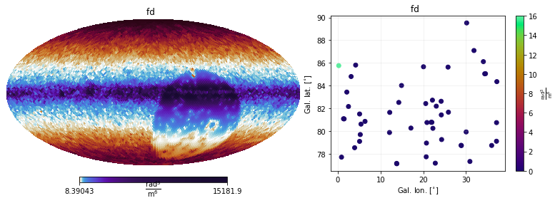
One may also be interested in visualising the associated covariance matrices, which in this case are diagonals, since the Dataset objects were initialized using the error keyword argument.
[15]:
plt.figure(figsize=(12,4))
mea.cov.show()

It is also possible to show only the variances (i.e. the diagonals of the covariance matrices). This is plotted as maps, to aid the interpretation
[16]:
plt.figure(figsize=(12,4))
mea.cov.show(show_variances=True)
Finally, to directly access the data, one needs first to find out what the keys are:
[17]:
list(mea.keys())
[17]:
[('fd', None, 32, None), ('fd', None, 'tab', None)]
and use them to get the data using the global_data property
[18]:
my_key = ('fd', None, 32, None)
extracted_obs_data = mea[my_key].global_data

print(type(extracted_obs_data))
print(extracted_obs_data.shape)
<class 'numpy.ndarray'>
(1, 12288)
The property global_data automatically gathers the data if rc['distributed_arrays'] is set to True, while the attribute data returns the local values. If not using 'distributed_arrays' the two options are equivalent.
Manually appending data
An alternative way to include data into an Observables dictionary is explicitly choosing the key and adjusting the data shape. One can see how this is handled by the Dataset object in the following cell
[19]:
# Creates a new dataset
dset = FaradayDepthOppermann2012(Nside=2)
# This is how HEALPix data can be included without the mediation of Datasets:
cov = np.diag(dset.var)  # Covariance matrix from the variances
mea.append(name=dset.key, data=dset.data, cov_data=cov, otype='HEALPix')
# This is what Dataset is doing:
print('The key used in the "name" arg was:', dset.key)
print('The shape of data was:', dset.data.shape)
print('The shape of the covariance matrix arg was:', cov.shape)
The key used in the "name" arg was: ('fd', None, 2, None)
The shape of data was: (1, 48)
The shape of the covariance matrix arg was: (48, 48)
But what exactly is stored in mea? This is handled by an Observable object. Here we illustrate with the tabular dataset previously defined.
[20]:
print(type(mea[dset_tab.key]))
print('mea.data:', repr(mea[dset_tab.key].data))
print('mea.data.shape:', mea[dset_tab.key].data.shape)
print('mea.unit', repr(mea[dset_tab.key].unit))
print('mea.coords (coordinates dict -- for tabular datasets only):\n',
      mea[dset_tab.key].coords)
print('mea.dtype:', mea[dset_tab.key].dtype)
print('mea.otype:', mea[dset_tab.key].otype)
print('\n\nmea.cov type',type(mea.cov[dset_tab.key]))
print('mea.cov.data type:', type(mea.cov[dset_tab.key].data))
print('mea.cov.data.shape:', mea.cov[dset_tab.key].data.shape)
print('mea.cov.dtype:', mea.cov[dset_tab.key].dtype)
<class 'imagine.observables.observable.Observable'>
mea.data: array([[ -3.,   3.,  -6.,   0.,   4.,  -6.,   5.,  -1.,  -6.,   1., -14.,
         14.,   3.,  10.,  12.,  16.,  -3.,   5.,  12.,   6.,  -1.,   5.,
          5.,  -4.,  -1.,   9.,  -1., -13.,   4.,   5.,  -5.,  17., -10.,
          8.,   0.,   1.,   5.,   9.,   5., -12., -17.,   4.,   2.,  -1.,
         -3.,   3.,  16.,  -1.,  -1.,   3.]])
mea.data.shape: (1, 50)
mea.unit Unit("rad / m2")
mea.coords (coordinates dict -- for tabular datasets only):
 {'type': 'galactic', 'lon': <Quantity [ 0.21,  0.86,  1.33,  1.47,  2.1 ,  2.49,  3.11,  3.93,  4.17,
            5.09,  5.09,  5.25,  5.42,  6.36, 12.09, 12.14, 13.76, 13.79,
           14.26, 14.9 , 17.1 , 20.04, 20.56, 20.67, 20.73, 20.85, 21.83,
           22.  , 22.13, 22.24, 22.8 , 23.03, 24.17, 24.21, 24.28, 25.78,
           25.87, 28.84, 28.9 , 30.02, 30.14, 30.9 , 31.85, 34.05, 34.37,
           34.54, 35.99, 37.12, 37.13, 37.2 ] deg>, 'lat': <Quantity [85.76, 77.7 , 81.08, 81.07, 83.43, 82.16, 84.8 , 78.53, 85.81,
           79.09, 81.5 , 79.69, 80.61, 80.85, 79.87, 81.64, 77.15, 77.12,
           82.52, 84.01, 80.26, 85.66, 82.42, 77.73, 78.94, 80.75, 80.77,
           80.77, 82.72, 80.24, 77.17, 82.19, 82.62, 81.42, 79.25, 85.63,
           81.66, 78.74, 78.72, 79.92, 89.52, 77.32, 87.09, 86.11, 85.04,
           85.05, 78.73, 79.1 , 80.74, 84.35] deg>}
mea.dtype: measured
mea.otype: tabular


mea.cov type <class 'imagine.observables.observable.Observable'>
mea.cov.data type: <class 'numpy.ndarray'>
mea.cov.data.shape: (50, 50)
mea.cov.dtype: variance
The Dataset object may also automatically distribute the data across different nodes if one is running the code using MPI parallelisation – a strong reason for sticking to using Datasets instead of appending directly.