Basic elements of an IMAGINE pipeline

In this tutorial, we focus on introducing the basic building blocks of the IMAGINE package and how to use them for assembling a Bayesian analysis pipeline.

We will use mock data with only two independent free parameters. First, we will generate the mock data. Then we will assemble all elements needed for the IMAGINE pipeline, execute the pipeline and investigate its results.

The mock data are designed to “naively” mimic Faraday depth, which is affected linearly by the (Galactic) magnetic field and thermal electron density. As a function of position \(x\), we define a constant coherent magnetic field component \(a_0\) and a random magnetic field component which is drawn from a Gaussian distribution with standard deviation \(b_0\). The electron density is assumed to be independently known and given by a \(\cos(x)\) with arbitrary scaling. The mock data values we get are related to the Faraday depth of a background source at some arbitrary distance:

\[signal(x) = \left[1+\cos(x)\right] \times \mathcal{G}(\mu=a_0,\sigma=b_0;seed=s)\,{\mu\rm G\,cm}^{-3} , \; x \in [0,2\pi]\,\rm kpc\]

where \(\{a_0,b_0\}\) is the ‘physical’ parameter set, and \(s\) represents the seed for random variable generation.

The purpose is not to fit the exact signal, since it includes a stochastic component, but to fit the amplitude of the signal and of the variations around it. So this is fitting the strength of the coherent field \(a_0\) and the amplitude of the random field \(b_0\). With these mock data and its (co)variance matrix, we shall assemble the IMAGINE pipeline, execute it and examine its results.

First, import the necessary packages.

import numpy as np
import astropy.units as u
import astropy as apy
import matplotlib.pyplot as plt

import imagine as img

%matplotlib inline

1) Preparing the mock data

In calculating the mock data values, we introduce noise as:

\[data(x) = signal(x) + noise(x)\]

For simplicity, we propose a simple gaussian noise with mean zero and a standard deviation \(e\):

\[noise(x) = \mathcal{G}(\mu=0,\sigma=e)\]

.

We will assume that we have 10 points in the x-direction, in the range \([0, 2\pi]\,\rm kpc\).

a0 = 3. # true value of a in microgauss
b0 = 6. # true value of b in microgauss
e = 0.1 # std of gaussian measurement error
s = 233 # seed fixed for signal field

size = 10 # data size in measurements
x = np.linspace(0.01,2.*np.pi-0.01,size) # where the observer is looking at

np.random.seed(s) # set seed for signal field

signal = (1+np.cos(x)) * np.random.normal(loc=a0,scale=b0,size=size)

fd = signal + np.random.normal(loc=0.,scale=e,size=size)

# We load these to an astropy table for illustration/visualisation
data = apy.table.Table({'meas' : u.Quantity(fd, u.microgauss*u.cm**-3),
                  'err': np.ones_like(fd)*e,
                  'x': x,
                  'y': np.zeros_like(fd),
                  'z': np.zeros_like(fd),
                  'other': np.ones_like(fd)*42})
data[:4] # Shows the first 4 points in tabular form

Table length=4

meas	err	x	y	z	other
uG / cm3
float64	float64	float64	float64	float64	float64
16.4217790817552	0.1	0.01	0.0	0.0	42.0
7.172468731201507	0.1	0.7059094785755097	0.0	0.0	42.0
-3.2254947821460433	0.1	1.4018189571510193	0.0	0.0	42.0
0.27949334758966465	0.1	2.0977284357265287	0.0	0.0	42.0

These data need to be converted to an IMAGINE compatible format. To do this, we first create TabularDataset object, which helps importing dictionary-like dataset onto IMAGINE.

mockDataset = img.observables.TabularDataset(data, name='test',
                                             data_col='meas',
                                             err_col='err')

These lines simply explain how to read the tabular dataset (note that the ‘other’ column is ignored): name contains the type of observable we are using (here, we use ‘test’, it could also be ‘sync’ for synchrotron observables (e.g, Stokes parameters), ‘fd’ for Faraday Depth, etc. The data_col argument specifies the key or name of the column containing the relevant measurement. Coordinates (coords_type) can be given in either 'cartesian' or 'galactic'. If not provided, the coordinates type is derived from the provided data. In this example, we provided \(x\), \(y\) and \(z\) in \(\rm kpc\) and therefore the coordinates type is assumed to be ‘cartesian’. The units of the dataset are represented using astropy.units objects and can be supplied (if they are, the Simulator will later check whether these are adequate and automatically convert the data to other units if needed).

The dataset can be loaded onto a Measurements object, which is subclass of ObservableDict. This object allows one to supply multiple datasets to the pipeline.

# Create Measurements object using mockDataset
mock_data = img.observables.Measurements(mockDataset)

The dataset object creates a standard key for each appended dataset. In our case, there is only one key.

keys = list(mock_data.keys())
keys

[('test', None, 'tab', None)]

Let us plot the mock data as well as the \(1+\cos(x)\) function that is the underlying variation.

The property Measurements.global_data extracts arrays from the Observable object which is hosted inside the ObservableDict class.

plt.scatter(x, mock_data[keys[0]].global_data[0], marker='.', label='signal')
plt.plot(x,(1+np.cos(x))*a0,'r--',label='$1+\cos(x)$')
plt.xlabel('x'); plt.legend();

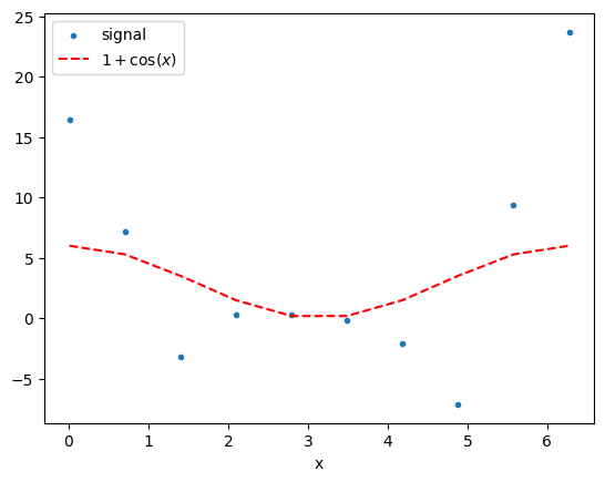
Note that the variance in the signal is highest where the \(\cos(x)\) is also strongest. This is the way we expect the Faraday depth to work, since a fluctuation in the strength of \(\mathbf B\) has a larger effect on the RM when \(n_e\) also happens to be higher.

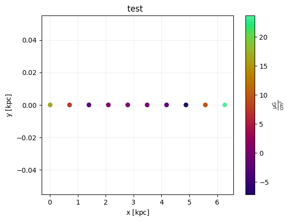
IMAGINE also comes with a built-in method for showing the contents of a Measurements objects on a skymap. In the next cell this is exemplified, though not very useful for this specific example.

mock_data.show(cartesian_axes='xy')

2) Pipeline assembly

Now that we have generated mock data, there are a few steps to set up the pipeline to estimate the input parameters. We need to specify: a grid, Field Factories, Simulators, and Likelihoods.

Setting the coordinate grid

Fields in IMAGINE represent models of any kind of physical field – in this particular tutorial, we will need a magnetic field and thermal electron density.

The Fields are evaluated on a grid of coordinates, represented by a img.Grid object. Here we exemplify how to produce a regular cartesian grid. To do so, we need to specify the values of the coordinates on the 6 extremities of the box (i.e. the minimum and maximum value for each coordinate), and the resolution over each dimension.

For this particular artificial example, we actually only need one dimension, so we set the resolution to 1 for \(y\) and \(z\).

one_d_grid = img.fields.UniformGrid(box=[[0,2*np.pi]*u.kpc,
                                         [0,0]*u.kpc,
                                         [0,0]*u.kpc],
                                    resolution=[30,1,1])

Preparing the Field Factory list

A particular realisation of a model for a physical field is represented within IMAGINE by a Field object, which, given set of parameters, evaluates the field for over the grid.

A Field Factory is an associated piece of infrastructure used by the Pipeline to produce new Fields. It is a Factory object that needs to be initialized and supplied to the Pipeline. This is what we will illustrate here.

from imagine import fields
ne_factory = fields.CosThermalElectronDensityFactory(grid=one_d_grid)

The previous line instantiates CosThermalElectronDensityFactory with the previously defined Grid object. This Factory allows the Pipeline to produce CosThermalElectronDensity objects. These correspond to a toy model for electron density with the form:

\[n_e(x,y,z) = n_0 [1+\cos (a x + \alpha)][1+\cos (b y + \beta)][1+\cos(c z + \gamma)]\,.\]

We can set and check the default parameter values in the following way:

ne_factory.default_parameters= {'a': 1*u.rad/u.kpc,
                                'beta':  np.pi/2*u.rad,
                                'gamma': np.pi/2*u.rad}
ne_factory.default_parameters

{'n0': <Quantity 1. 1 / cm3>,
 'a': <Quantity 1. rad / kpc>,
 'b': <Quantity 0. rad / kpc>,
 'c': <Quantity 0. rad / kpc>,
 'alpha': <Quantity 0. rad>,
 'beta': <Quantity 1.57079633 rad>,
 'gamma': <Quantity 1.57079633 rad>}

ne_factory.active_parameters

()

For ne_factory, no active parameters were set. This means that the Field will be always evaluated using the specified default parameter values.

We will now similarly define the magnetic field, using the NaiveGaussianMagneticField which constructs a “naive” random field (i.e. the magnitude of \(x\), \(y\) and \(z\) components of the field are drawn from a Gaussian distribution without imposing zero divergence, thus do not use this for serious applications).

B_factory = fields.NaiveGaussianMagneticFieldFactory(grid=one_d_grid)

Differently from the case of ne_factory, in this case we would like to make the parameters active. All individual components of the field are drawn from a Gaussian distribution with mean \(a_0\) and standard deviation \(b_0\). To set these parameters as active we do:

B_factory.active_parameters = ('a0','b0')
B_factory.priors ={'a0': img.priors.FlatPrior(xmin=-4*u.microgauss,
                                              xmax=5*u.microgauss),
                   'b0': img.priors.FlatPrior(xmin=2*u.microgauss,
                                              xmax=10*u.microgauss)}

In the lines above we chose uniform (flat) priors for both parameters within the above specified ranges. Any active parameter must have a Prior distribution specified.

Once the two FieldFactory objects are prepared, they put together in a list which is later supplied to the Pipeline.

factory_list = [ne_factory, B_factory]

Initializing the Simulator

For this tutorial, we use a customized TestSimulator which simply computes the quantity: \(t(x,y,z) = B_y\,n_e\,\),i.e. the contribution at one specific point to the Faraday depth.

The simulator is initialized with the mock Measurements defined before, which allows it to know what is the correct format for output.

from imagine.simulators import TestSimulator
simer = TestSimulator(mock_data)

Initializing the Likelihood

IMAGINE provides the Likelihood class with EnsembleLikelihood and SimpleLikelihood as two options. The SimpleLikelihood is what you expect, computing a single \(\chi^2\) from the difference of the simulated and the measured datasets. The EnsembleLikelihood is how IMAGINE handles a signal which itself includes a stochastic component, e.g., what we call the Galactic variance. This likelihood module makes use of a finite ensemble of simulated realizations and uses their mean and covariance to compare them to the measured dataset.

likelihood = img.likelihoods.EnsembleLikelihood(mock_data)

3) Running the pipeline

Now we have all the necessary components available to run our pipeline. This can be done through a Pipeline object, which interfaces with some algorithm to sample the likelihood space accounting for the prescribed prior distributions for the parameters.

IMAGINE comes with a range of samplers coded as different Pipeline classes, most of which are based on the nested sampling approach. In what follows we will use the MultiNest sampler as an example.

IMAGINE takes care of stochastic fields by evaluating an ensemble of random realisations for each selected point in the parameter space, and computing the associated covariance (i.e. estimating the Galactic variance). We can set this up through the ensemble_size argument.

Now we are ready to initialize our final pipeline.

pipeline = img.pipelines.MultinestPipeline(simulator=simer,
                                           run_directory='../runs/tutorial_one',
                                           factory_list=factory_list,
                                           likelihood=likelihood,
                                           ensemble_size=27)

The run_directory keyword is used to setup where the state of the pipeline is saved (allowing loading the pipeline in the future). It is also where the chains generated by the sampler are saved in the sampler’s native format (if the sampler supports this).

The property sampling_controllers allows one to send sampler-specific parameters to the chosen Pipeline. Each IMAGINE Pipeline object will have slightly different sampling controllers, which can be found in the specific Pipeline’s docstring.

pipeline.sampling_controllers = {'evidence_tolerance': 0.5, 'n_live_points': 200}

In a standard nested sampling approach, a set of “live points” is initially sampled from the prior distribution. After each iteration the point with the smallest likelihood is removed (it becomes a dead point, and its likelihood value is stored) and a new point is sampled from the prior. As each dead point is associated to some prior volume, they can be used to estimate the evidence (see, e.g. here for details). In the MultinestPipeline, the number of live points is set using the 'n_live_points' sampling controller.

The sampling parameter 'evidence_tolerance' allows one to control the target error in the estimated evidence.

Now, we finally can run the pipeline!

results = pipeline()

 *****************************************************
 MultiNest v3.10
 Copyright Farhan Feroz & Mike Hobson
 Release Jul 2015

 no. of live points =  200
 dimensionality =    2
 resuming from previous job
 *****************************************************
 Starting MultiNest
Acceptance Rate:                        0.798156
Replacements:                                779
Total Samples:                               976
Nested Sampling ln(Z):                -34.103959
Importance Nested Sampling ln(Z):     -33.834852 +/-  0.017866
  analysing data from ../runs/tutorial_one/chains/multinest_.txt
 ln(ev)=  -33.740333744870789      +/-   6.8554728937079146E-002
 Total Likelihood Evaluations:          976
 Sampling finished. Exiting MultiNest

Posterior report:

$\displaystyle \\ \text{ naive_gaussian_magnetic_field_a0: }\; 3.1^{+1.2}_{-2.1}\,\mathrm{\mu G}\\\\ \text{ naive_gaussian_magnetic_field_b0: }\; 6.1^{+1.6}_{-1.1}\,\mathrm{\mu G}\\$

Evidence report:

$\displaystyle \log\mathcal{{ Z }} = -33.74\pm 0.07$

Thus, one can see that after the pipeline finishes running, a brief summary report is written to screen.

When one runs the pipeline it returns a results dictionary object in the native format of the chosen sampler. Alternatively, after running the pipeline object, the results can also be accessed through its attributes, which are standard interfaces (i.e. all pipelines should work in the same way).

For comparing different models, the quantity of interest is the model evidence (or marginal likelihood) \(\mathcal Z\). After a run, this can be easily accessed as follows.

print('log evidence: {0:.2f} ± {1:.2f}'.format(pipeline.log_evidence,
                                               pipeline.log_evidence_err))

log evidence: -33.74 ± 0.07

A dictionary containing a summary of the constraints to the parameters can be accessed through the property posterior_summary:

pipeline.posterior_summary

{'naive_gaussian_magnetic_field_a0': {'median': <Quantity 3.0814833 uG>,
  'errlo': <Quantity 2.05593751 uG>,
  'errup': <Quantity 1.20576586 uG>,
  'mean': <Quantity 2.69388628 uG>,
  'stdev': <Quantity 1.63193297 uG>},
 'naive_gaussian_magnetic_field_b0': {'median': <Quantity 6.0654585 uG>,
  'errlo': <Quantity 1.12518132 uG>,
  'errup': <Quantity 1.58336481 uG>,
  'mean': <Quantity 6.25303211 uG>,
  'stdev': <Quantity 1.34689108 uG>}}

In most cases, however, one would (should) prefer to work directly on the samples produced by the sampler. A table containing the parameter values of the samples generated can be accessed through:

samples = pipeline.samples
samples[:3] # Displays only first 3 rows

QTable length=3

naive_gaussian_magnetic_field_a0	naive_gaussian_magnetic_field_b0
uG	uG
float64	float64
0.09251022338867188	3.9516048431396484
-2.5668919682502747	5.735667705535889
-3.9131999611854553	8.597143173217773

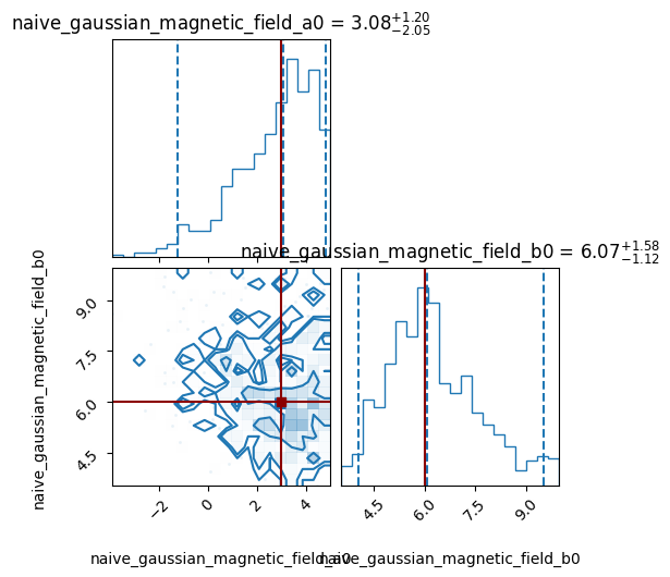
For convenience, the corner plot showing the posterior distribution obtained from the samples can be generated using the corner_plot method of the Pipeline object (which uses the corner library). This can show “truth” values of the parameters (in case someone is doing a test like this one).

pipeline.corner_plot(truths_dict={'naive_gaussian_magnetic_field_a0': 3,
                                  'naive_gaussian_magnetic_field_b0': 6});

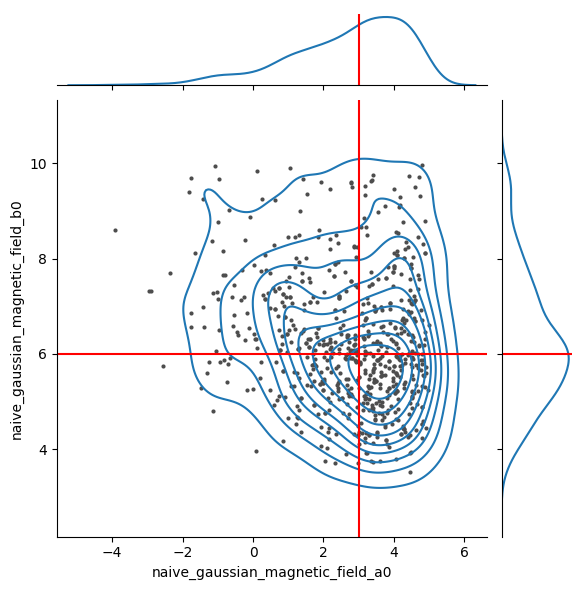
One can, of course, choose other plotting/analysis routines. Below, the use of seaborn is exemplified.

import seaborn as sns
def plot_samples_seaborn(samp):

    def show_truth_in_jointplot(jointplot, true_x, true_y, color='r'):
        for ax in (jointplot.ax_joint, jointplot.ax_marg_x):
            ax.vlines([true_x], *ax.get_ylim(), colors=color)
        for ax in (jointplot.ax_joint, jointplot.ax_marg_y):
            ax.hlines([true_y], *ax.get_xlim(), colors=color)

    snsfig = sns.jointplot(samp.to_pandas(), x=samp.colnames[0], y=samp.colnames[1], kind='kde')
    snsfig.plot_joint(sns.scatterplot, linewidth=0, marker='.', color='0.3')
    show_truth_in_jointplot(snsfig, a0, b0)

plot_samples_seaborn(samples)

Random seeds and convergence checks

The pipeline relies on random numbers in multiple ways. The Monte Carlo sampler will draw randomly chosen points in the parameter space duing its exploration (in the specific case of nested sampling pipelines, these are drawn from the prior distributions). Also, while evaluating the fields at each point, random realisations of the stochastic fields are generated.

It is possible to control the behaviour of the random seeding of an IMAGINE pipeline through the attribute master_seed. This attribute has two uses: it is passed to the sampler, ensuring that its behaviour is reproducible; and it is also used to generate a fresh list of new random seeds to each stochastic field that is evaluated.

pipeline.master_seed

1

By default, the master seed is fixed and set to 1, but you can alter its value before running the pipeline.

One can also change the seeding behaviour through the random_type attribute. There are three allowed options for this:

• ‘controllable’ - the master_seed is constant and a re-running the pipeline should lead to the exact same results (default), and the random seeds which are used for generating the ensembles of stochastic fields are drawn in the beginning of the pipeline run;
• ‘free’ - on each execution, a new master_seed is drawn (using numpy.randint), moreover: at each evaluation of the likelihood the stochastic fields receive a new set of ensemble seeds;
• ‘fixed’ - this mode is for debugging purposes. The master_seed is fixed, as in the ‘controllable’ case, however each individual stochastic field receives the exact same list of ensemble seeds every time (while in the controllable these are chosen “randomly” at run-time). Such choice can be inspected using pipeline.ensemble_seeds.

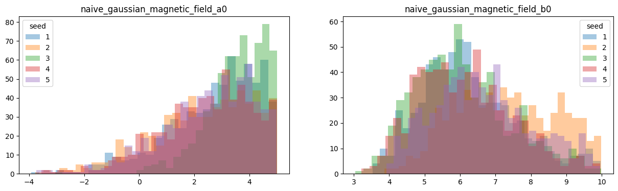
Let us now check whether different executions of the pipeline are generating consistent results. To do so, we run it five times and just overplot histograms of the outputs to see if they all look the same. The following can be done in a few minutes.

fig, axs = plt.subplots(1, 2, figsize=(15, 4))
repeat = 5
pipeline.show_summary_reports = False  # Avoid summary reports
pipeline.sampling_controllers['resume'] = False # Pipeline will re-run
samples_list = []
for i in range(1,repeat+1):
    print('-'*60+'\nRun {}/{}'.format(i,repeat))
    if i>1:
        # Re-runs the pipeline with a different seed
        pipeline.master_seed = i
        _ = pipeline()
    print('log Z = ', round(pipeline.log_evidence,4),
          '±', round(pipeline.log_evidence_err,4))

    samples = pipeline.samples

    for j, param in enumerate(pipeline.samples.columns):
        samp = samples[param]
        axs[j].hist(samp.value, alpha=0.4, bins=30, label=pipeline.master_seed)
        axs[j].set_title(param)
    # Stores the samples for later use
    samples_list.append(samples)

for i in range(2):
    axs[i].legend(title='seed')

------------------------------------------------------------
Run 1/5
log Z =  -33.7403 ± 0.0686
------------------------------------------------------------
Run 2/5
 *****************************************************
 MultiNest v3.10
 Copyright Farhan Feroz & Mike Hobson
 Release Jul 2015

 no. of live points =  200
 dimensionality =    2
 *****************************************************
 Starting MultiNest
 generating live points
 live points generated, starting sampling
Acceptance Rate:                        0.976562
Replacements:                                250
Total Samples:                               256
Nested Sampling ln(Z):                -45.666321
Importance Nested Sampling ln(Z):     -36.404469 +/-  0.075459
Acceptance Rate:                        0.895522
Replacements:                                300
Total Samples:                               335
Nested Sampling ln(Z):                -40.635040
Importance Nested Sampling ln(Z):     -36.407765 +/-  0.067082
Acceptance Rate:                        0.870647
Replacements:                                350
Total Samples:                               402
Nested Sampling ln(Z):                -39.285136
Importance Nested Sampling ln(Z):     -36.454334 +/-  0.058365
Acceptance Rate:                        0.875274
Replacements:                                400
Total Samples:                               457
Nested Sampling ln(Z):                -38.408561
Importance Nested Sampling ln(Z):     -36.494367 +/-  0.050070
Acceptance Rate:                        0.855513
Replacements:                                450
Total Samples:                               526
Nested Sampling ln(Z):                -37.871122
Importance Nested Sampling ln(Z):     -36.549895 +/-  0.041256
Acceptance Rate:                        0.846024
Replacements:                                500
Total Samples:                               591
Nested Sampling ln(Z):                -37.513938
Importance Nested Sampling ln(Z):     -36.544110 +/-  0.034267
Acceptance Rate:                        0.838415
Replacements:                                550
Total Samples:                               656
Nested Sampling ln(Z):                -37.269002
Importance Nested Sampling ln(Z):     -36.532255 +/-  0.028526
Acceptance Rate:                        0.831025
Replacements:                                600
Total Samples:                               722
Nested Sampling ln(Z):                -37.082216
Importance Nested Sampling ln(Z):     -36.515849 +/-  0.024415
Acceptance Rate:                        0.829082
Replacements:                                650
Total Samples:                               784
Nested Sampling ln(Z):                -36.937410
Importance Nested Sampling ln(Z):     -36.505272 +/-  0.021148
Acceptance Rate:                        0.824499
Replacements:                                700
Total Samples:                               849
Nested Sampling ln(Z):                -36.824190
Importance Nested Sampling ln(Z):     -36.493166 +/-  0.018719
Acceptance Rate:                        0.829519
Replacements:                                725
Total Samples:                               874
Nested Sampling ln(Z):                -36.776663
Importance Nested Sampling ln(Z):     -36.487902 +/-  0.017987
 ln(ev)=  -36.422024811734140      +/-   5.9904573990813136E-002
 Total Likelihood Evaluations:          874
 Sampling finished. Exiting MultiNest
  analysing data from ../runs/tutorial_one/chains/multinest_.txt
log Z =  -36.422 ± 0.0599
------------------------------------------------------------
Run 3/5
 *****************************************************
 MultiNest v3.10
 Copyright Farhan Feroz & Mike Hobson
 Release Jul 2015

 no. of live points =  200
 dimensionality =    2
 *****************************************************
 Starting MultiNest
 generating live points
 live points generated, starting sampling
Acceptance Rate:                        0.961538
Replacements:                                250
Total Samples:                               260
Nested Sampling ln(Z):                -47.812896
Importance Nested Sampling ln(Z):     -33.614487 +/-  0.124036
Acceptance Rate:                        0.906344
Replacements:                                300
Total Samples:                               331
Nested Sampling ln(Z):                -41.071707
Importance Nested Sampling ln(Z):     -33.584705 +/-  0.103246
Acceptance Rate:                        0.825472
Replacements:                                350
Total Samples:                               424
Nested Sampling ln(Z):                -38.845330
Importance Nested Sampling ln(Z):     -33.682256 +/-  0.091810
Acceptance Rate:                        0.813008
Replacements:                                400
Total Samples:                               492
Nested Sampling ln(Z):                -37.336397
Importance Nested Sampling ln(Z):     -33.779787 +/-  0.079815
Acceptance Rate:                        0.809353
Replacements:                                450
Total Samples:                               556
Nested Sampling ln(Z):                -36.258290
Importance Nested Sampling ln(Z):     -33.765373 +/-  0.068468
Acceptance Rate:                        0.797448
Replacements:                                500
Total Samples:                               627
Nested Sampling ln(Z):                -35.614828
Importance Nested Sampling ln(Z):     -33.792933 +/-  0.058122
Acceptance Rate:                        0.784593
Replacements:                                550
Total Samples:                               701
Nested Sampling ln(Z):                -35.171530
Importance Nested Sampling ln(Z):     -33.816602 +/-  0.048070
Acceptance Rate:                        0.789474
Replacements:                                600
Total Samples:                               760
Nested Sampling ln(Z):                -34.819673
Importance Nested Sampling ln(Z):     -33.815325 +/-  0.041250
Acceptance Rate:                        0.793651
Replacements:                                650
Total Samples:                               819
Nested Sampling ln(Z):                -34.561405
Importance Nested Sampling ln(Z):     -33.793241 +/-  0.035470
Acceptance Rate:                        0.790960
Replacements:                                700
Total Samples:                               885
Nested Sampling ln(Z):                -34.353055
Importance Nested Sampling ln(Z):     -33.799881 +/-  0.029433
Acceptance Rate:                        0.789474
Replacements:                                750
Total Samples:                               950
Nested Sampling ln(Z):                -34.185075
Importance Nested Sampling ln(Z):     -33.808944 +/-  0.024665
Acceptance Rate:                        0.780488
Replacements:                                800
Total Samples:                              1025
Nested Sampling ln(Z):                -34.053277
Importance Nested Sampling ln(Z):     -33.815633 +/-  0.020893
Acceptance Rate:                        0.776761
Replacements:                                849
Total Samples:                              1093
Nested Sampling ln(Z):                -33.951214
Importance Nested Sampling ln(Z):     -33.814557 +/-  0.018646
 ln(ev)=  -33.593024067542828      +/-   7.8769977225718352E-002
 Total Likelihood Evaluations:         1093
 Sampling finished. Exiting MultiNest
  analysing data from ../runs/tutorial_one/chains/multinest_.txt
log Z =  -33.593 ± 0.0788
------------------------------------------------------------
Run 4/5
 *****************************************************
 MultiNest v3.10
 Copyright Farhan Feroz & Mike Hobson
 Release Jul 2015

 no. of live points =  200
 dimensionality =    2
 *****************************************************
 Starting MultiNest
 generating live points
 live points generated, starting sampling
Acceptance Rate:                        0.957854
Replacements:                                250
Total Samples:                               261
Nested Sampling ln(Z):                -43.912707
Importance Nested Sampling ln(Z):     -33.364001 +/-  0.085718
Acceptance Rate:                        0.920245
Replacements:                                300
Total Samples:                               326
Nested Sampling ln(Z):                -37.883027
Importance Nested Sampling ln(Z):     -33.352252 +/-  0.074666
Acceptance Rate:                        0.870647
Replacements:                                350
Total Samples:                               402
Nested Sampling ln(Z):                -36.400320
Importance Nested Sampling ln(Z):     -33.320058 +/-  0.064325
Acceptance Rate:                        0.849257
Replacements:                                400
Total Samples:                               471
Nested Sampling ln(Z):                -35.548976
Importance Nested Sampling ln(Z):     -33.370917 +/-  0.054626
Acceptance Rate:                        0.841121
Replacements:                                450
Total Samples:                               535
Nested Sampling ln(Z):                -34.988318
Importance Nested Sampling ln(Z):     -33.405821 +/-  0.045581
Acceptance Rate:                        0.840336
Replacements:                                500
Total Samples:                               595
Nested Sampling ln(Z):                -34.606288
Importance Nested Sampling ln(Z):     -33.449831 +/-  0.037749
Acceptance Rate:                        0.835866
Replacements:                                550
Total Samples:                               658
Nested Sampling ln(Z):                -34.312554
Importance Nested Sampling ln(Z):     -33.452185 +/-  0.031043
Acceptance Rate:                        0.836820
Replacements:                                600
Total Samples:                               717
Nested Sampling ln(Z):                -34.084872
Importance Nested Sampling ln(Z):     -33.457736 +/-  0.025515
Acceptance Rate:                        0.838710
Replacements:                                650
Total Samples:                               775
Nested Sampling ln(Z):                -33.910893
Importance Nested Sampling ln(Z):     -33.451359 +/-  0.021352
Acceptance Rate:                        0.831354
Replacements:                                700
Total Samples:                               842
Nested Sampling ln(Z):                -33.776988
Importance Nested Sampling ln(Z):     -33.449316 +/-  0.017841
Acceptance Rate:                        0.825942
Replacements:                                745
Total Samples:                               902
Nested Sampling ln(Z):                -33.683834
Importance Nested Sampling ln(Z):     -33.443333 +/-  0.015835
 ln(ev)=  -33.329049708696836      +/-   6.3601386661158138E-002
 Total Likelihood Evaluations:          902
 Sampling finished. Exiting MultiNest
  analysing data from ../runs/tutorial_one/chains/multinest_.txt
log Z =  -33.329 ± 0.0636
------------------------------------------------------------
Run 5/5
 *****************************************************
 MultiNest v3.10
 Copyright Farhan Feroz & Mike Hobson
 Release Jul 2015

 no. of live points =  200
 dimensionality =    2
 *****************************************************
 Starting MultiNest
 generating live points
 live points generated, starting sampling
Acceptance Rate:                        0.957854
Replacements:                                250
Total Samples:                               261
Nested Sampling ln(Z):                -46.152330
Importance Nested Sampling ln(Z):     -34.646650 +/-  0.087474
Acceptance Rate:                        0.911854
Replacements:                                300
Total Samples:                               329
Nested Sampling ln(Z):                -39.815741
Importance Nested Sampling ln(Z):     -34.683348 +/-  0.079590
Acceptance Rate:                        0.841346
Replacements:                                350
Total Samples:                               416
Nested Sampling ln(Z):                -38.244557
Importance Nested Sampling ln(Z):     -34.693583 +/-  0.070018
Acceptance Rate:                        0.785855
Replacements:                                400
Total Samples:                               509
Nested Sampling ln(Z):                -37.095894
Importance Nested Sampling ln(Z):     -34.674607 +/-  0.060084
Acceptance Rate:                        0.775862
Replacements:                                450
Total Samples:                               580
Nested Sampling ln(Z):                -36.449507
Importance Nested Sampling ln(Z):     -34.661885 +/-  0.049467
Acceptance Rate:                        0.778816
Replacements:                                500
Total Samples:                               642
Nested Sampling ln(Z):                -36.027403
Importance Nested Sampling ln(Z):     -34.643742 +/-  0.042104
Acceptance Rate:                        0.774648
Replacements:                                550
Total Samples:                               710
Nested Sampling ln(Z):                -35.720432
Importance Nested Sampling ln(Z):     -34.634377 +/-  0.034903
Acceptance Rate:                        0.780234
Replacements:                                600
Total Samples:                               769
Nested Sampling ln(Z):                -35.477838
Importance Nested Sampling ln(Z):     -34.617251 +/-  0.029627
Acceptance Rate:                        0.784077
Replacements:                                650
Total Samples:                               829
Nested Sampling ln(Z):                -35.289694
Importance Nested Sampling ln(Z):     -34.611212 +/-  0.025150
Acceptance Rate:                        0.784753
Replacements:                                700
Total Samples:                               892
Nested Sampling ln(Z):                -35.143225
Importance Nested Sampling ln(Z):     -34.614462 +/-  0.021699
Acceptance Rate:                        0.786988
Replacements:                                750
Total Samples:                               953
Nested Sampling ln(Z):                -35.032467
Importance Nested Sampling ln(Z):     -34.613896 +/-  0.019674
Acceptance Rate:                        0.787056
Replacements:                                754
Total Samples:                               958
Nested Sampling ln(Z):                -35.024913
Importance Nested Sampling ln(Z):     -34.614342 +/-  0.019554
 ln(ev)=  -34.665912282402459      +/-   6.6286044319899318E-002
 Total Likelihood Evaluations:          958
 Sampling finished. Exiting MultiNest
  analysing data from ../runs/tutorial_one/chains/multinest_.txt
log Z =  -34.6659 ± 0.0663

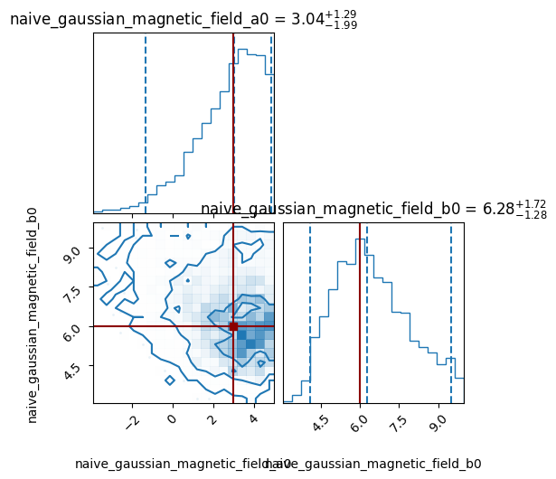
After being satisfied, one may want to put together all the samples. A set of rigorous tools for combining multiple pipelines/runs is currently under development, but a first order approximation to this can be seen below:

all_samples = apy.table.vstack(samples_list)
img.tools.corner_plot(table=all_samples,
                      truths_dict={'naive_gaussian_magnetic_field_a0': 3,
                                   'naive_gaussian_magnetic_field_b0': 6});

Script example

A script version of this tutorial can be found in the examples directory.